Principle Component Analysis Explained
What is Principle Component Analysis
Principal component analysis, or PCA, is a dimensionality reduction method that is often used to reduce the dimensionality of large data sets, by transforming a large set of variables into a smaller one that still contains most of the information in the large set.
Reducing the number of variables of a data set naturally comes at the expense of accuracy, but the trick in dimensionality reduction is to trade a little accuracy for simplicity. Because smaller data sets are easier to explore and visualize and make analyzing data points much easier and faster for machine learning algorithms without extraneous variables to process.
Standardization
The aim of this step is to standardize the range of the continuous initial variables so that each one of them contributes equally to the analysis.
More specifically, the reason why it is critical to perform standardization prior to PCA, is that the latter is quite sensitive regarding the variances of the initial variables. That is, if there are large differences between the ranges of initial variables, those variables with larger ranges will dominate over those with small ranges (for example, a variable that ranges between 0 and 100 will dominate over a variable that ranges between 0 and 1), which will lead to biased results. So, transforming the data to comparable scales can prevent this problem.
Mathematically, this can be done by subtracting the mean and dividing by the standard deviation for each value of each variable.
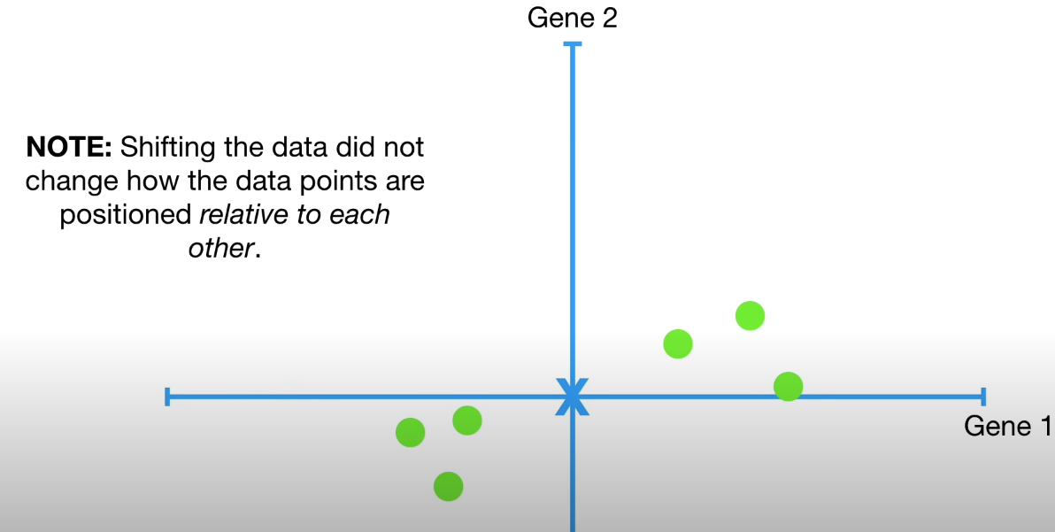
Shifting dataset to origin point does not scale the dataset.
Covariance Matrix Computation
The aim of this step is to understand how the variables of the input data set are varying from the mean with respect to each other, or in other words, to see if there is any relationship between them. Because sometimes, variables are highly correlated in such a way that they contain redundant information. So, in order to identify these correlations, we compute the covariance matrix.
The covariance matrix is a p × p symmetric matrix (where p is the number of dimensions) that has as entries the covariances associated with all possible pairs of the initial variables.
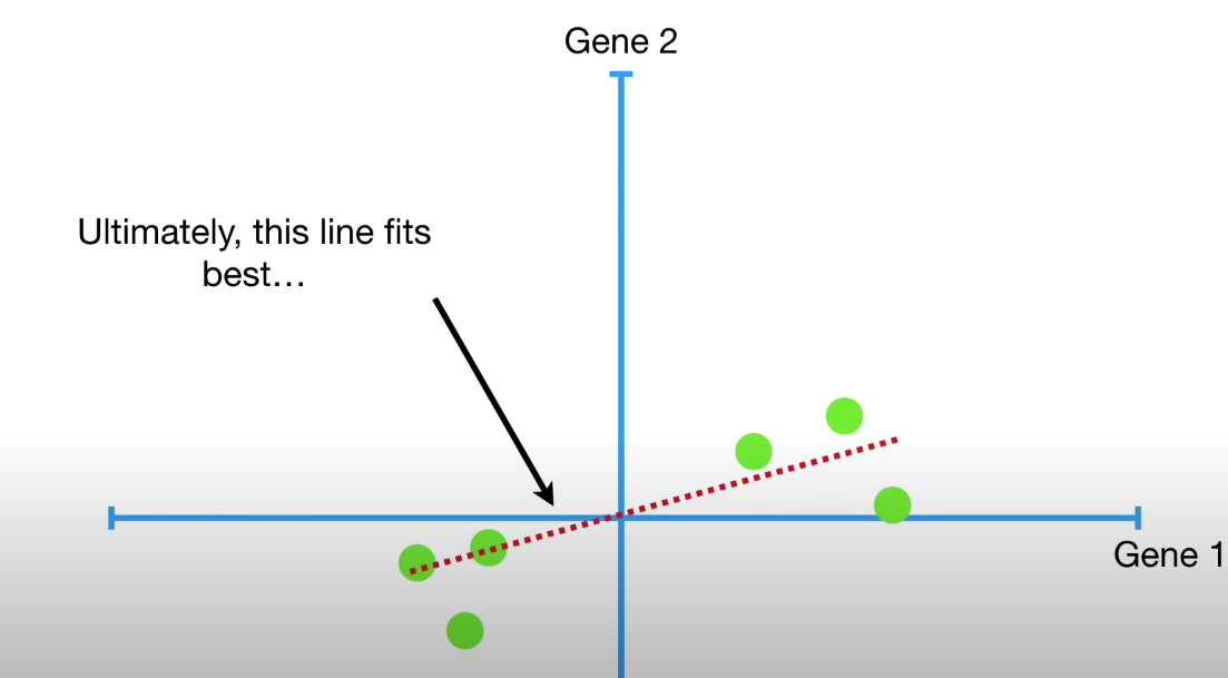
This ‘best fit line’ must go through the origin, and maximizes the sum of squared distances from the projected points to the origin.
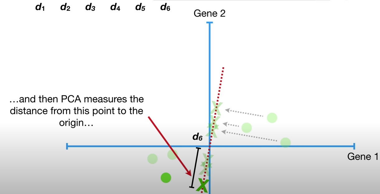
d1**2 + d2**2 + d3**2 + d4**2 + d5**2 + d6**2 = sum of squared distances = SS(distances)
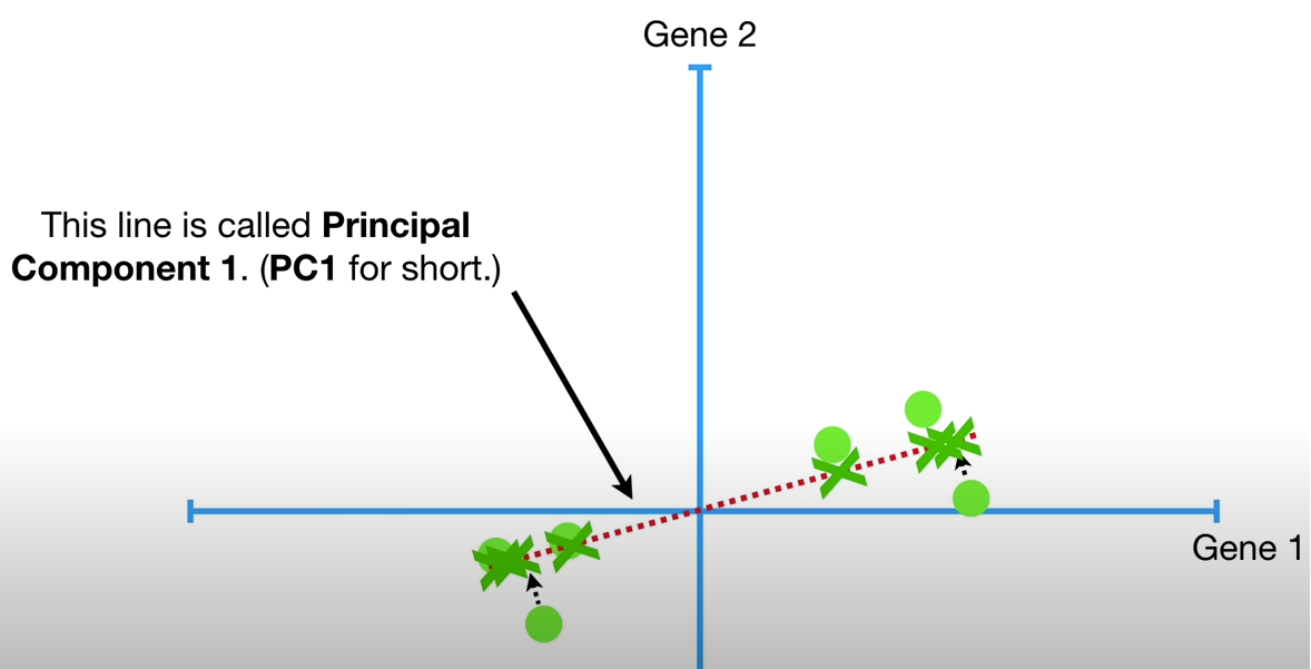
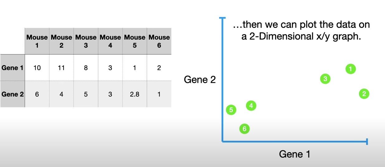
To make PC1, we need mix 4 parts Gene1 and 1 part Gene2, this is also called Linear Combination.
COMPUTE THE EIGENVECTORS AND EIGENVALUES OF THE COVARIANCE MATRIX TO IDENTIFY THE PRINCIPAL COMPONENTS
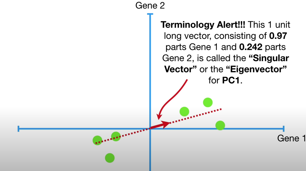
This 1 unit long vector, consisting of 0.97 parts Gene 1 and 0.242 parts of Gene 2, is called the Singular Vector or the Eigenvector for PC1.
To make PC1, mix 0.97 parts Gene1 with 0.242 parts Gene2, and the proportions of each gene are called Loading Scores.
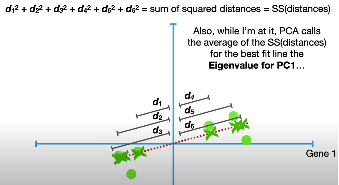
PCA calls the average of the SS(distances) for the best firt line the Eigenvalue for PC1
The square root of Eigenvalue is called Singular Value for PC1
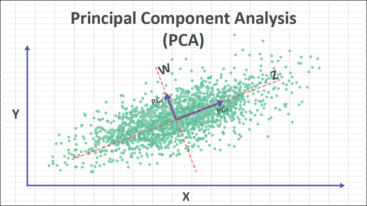
Eigenvectors and eigenvalues are the linear algebra concepts that we need to compute from the covariance matrix in order to determine the principal components of the data. Before getting to the explanation of these concepts, let’s first understand what do we mean by principal components.
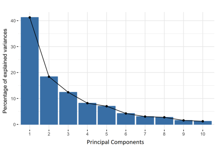
Principal components are new variables that are constructed as linear combinations or mixtures of the initial variables. These combinations are done in such a way that the new variables (i.e., principal components) are uncorrelated and most of the information within the initial variables is squeezed or compressed into the first components. So, the idea is 10-dimensional data gives you 10 principal components, but PCA tries to put maximum possible information in the first component, then maximum remaining information in the second and so on, until having something like shown in the scree plot below.
Variation for PC1 = SS(distances for PC1)/(n-1) Variation for PC2 = SS(distances for PC2)/(n-1)
PC1 accounts for Variation for PC1 / (Variation for PC1 + Variation for PC2) percentage of variables.
Feature Vector
As we saw in the previous step, computing the eigenvectors and ordering them by their eigenvalues in descending order, allow us to find the principal components in order of significance. In this step, what we do is, to choose whether to keep all these components or discard those of lesser significance (of low eigenvalues), and form with the remaining ones a matrix of vectors that we call Feature vector.
So, the feature vector is simply a matrix that has as columns the eigenvectors of the components that we decide to keep. This makes it the first step towards dimensionality reduction, because if we choose to keep only p eigenvectors (components) out of n, the final data set will have only p dimensions.
Recast The Data Along The Principle Components Axes
In the previous steps, apart from standardization, you do not make any changes on the data, you just select the principal components and form the feature vector, but the input data set remains always in terms of the original axes (i.e, in terms of the initial variables).
In this step, which is the last one, the aim is to use the feature vector formed using the eigenvectors of the covariance matrix, to reorient the data from the original axes to the ones represented by the principal components (hence the name Principal Components Analysis). This can be done by multiplying the transpose of the original data set by the transpose of the feature vector.
FinalDataset = FeatureVector.T * StandardizedOriginalDataset.T