Notes of Data Structures and Algorithms in Python
Recursion
Recursive functions typically follow this pattern:
- There are one or more base cases that are directly solvable without the need for further recursion.
- Each recursive call moves the solution progressively closer to a base case.
def factorial(n):
    return 1 if n <= 1 else n * factorial(n - 1)
import statistics
# Args: numbers is a list
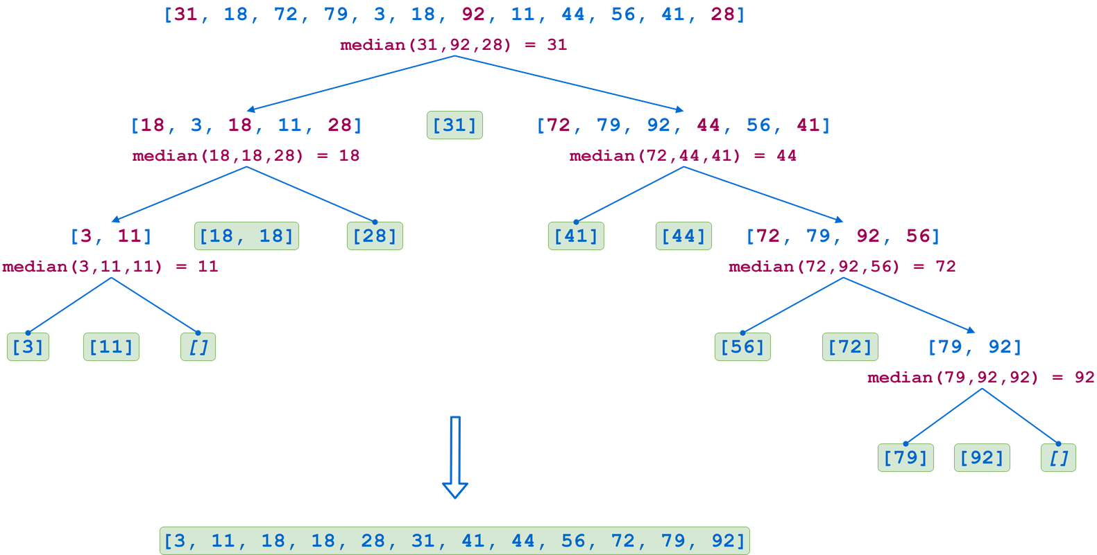
def quicksort(numbers: list = []) -> list:
# Base case
if len(numbers) <= 1:
return numbers
pivot = statistics.median(
[
numbers[0],
numbers[len(numbers) // 2],
numbers[-1]
]
)
items_less, pivot_items, items_greater = (
[n for n in numbers if n < pivot],
[n for n in numbers if n == pivot],
[n for n in numbers if n > pivot]
)
return (
quicksort(items_less) +
pivot_items +
quicksort(items_greater)
)
Linear Search VS Binary Search
In the case of linear search:
-
The time complexity of the algorithm is cN for some fixed constant c that depends on the number of operations we perform in each iteration and the time taken to execute a statement. Time complexity is sometimes also called the running time of the algorithm.
-
The space complexity is some constant c’ (independent of N), since we just need a single variable position to iterate through the array, and it occupies a constant spance in the computer’s memory(RAM).
Big O Notation: Worst-case complexity is often expressed using the Big O Notation, in the Big O, we drop fixed constants and lower powers of variables to capture the trend of relationship between the size of the input and the complexity of the algorithm i.e. if the complexity of the algorithm is cN^3 + dN^2 + eN + f, in the Big O notation it is expressed as O(N^3)
Thus, the time complexity of linear search is O(N) and its space complexity is O(1)
In the case of binary search:
k = log N
Where log refers to log to the base 2. Therefore, our algorithm has the time complexity O(log N). This fact is often stated as: binary search runs in logarithmic time. You can veify that the space complexity of binary search is O(1).
The real difference be tween the complexities: O(N) and O(log N)
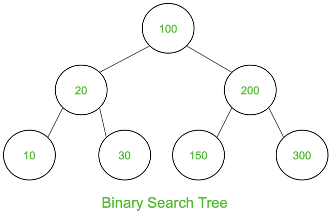
Binary Search Tree
A binary search tree (BST) is a node-based binary tree data structure that has the following properties.
- The left subtree of a node contains only nodes with keys less than the node’s key.
- The right subtree of a node contains only nodes with keys greater than the node’s key.
- Both the left and right subtrees must also be binary search trees.
- Each node (item in the tree) has a distinct key.
Binary Search Tree (BST) Traversals – Inorder, Preorder, Post Order
Output:
- Inorder Traversal: 10 20 30 100 150 200 300
- Preorder Traversal: 100 20 10 30 200 150 300
- Postorder Traversal: 10 30 20 150 300 200 100
Inorder Traversal:
At first traverse left subtree then visit the root and then traverse the right subtree.
- Traverse left subtree
- Visit the root and print the data.
- Traverse the right subtree
# Python3 code to implement the approach

# Class describing a node of tree
class Node:
    def __init__(self, v):
        self.left = None
        self.right = None
        self.data = v

# Inorder Traversal
def printInorder(root):
    if root:
        # Traverse left subtree
        printInorder(root.left)

        # Visit node <== Main different code
        print(root.data, end=" ")

        # Traverse right subtree
        printInorder(root.right)
Time complexity: O(N), Where N is the number of nodes. Auxiliary Space: O(h), Where h is the height of tree
Preorder Traversal:
At first visit the root then traverse left subtree and then traverse the right subtree.
- Visit the root and print the data.
- Traverse left subtree
- Traverse the right subtree
class Node:
    def __init__(self, v):
        self.data = v
        self.left = None
        self.right = None

# Preorder Traversal
def printPreOrder(node):
    if node is None:
        return
    # Visit Node <== Main different code
    print(node.data, end=" ")

    # Traverse left subtree
    printPreOrder(node.left)

    # Traverse right subtree
    printPreOrder(node.right)
Time complexity: O(N), Where N is the number of nodes. Auxiliary Space: O(H), Where H is the height of the tree
Postorder Traversal:
At first traverse left subtree then traverse the right subtree and then visit the root.
- Traverse left subtree
- Traverse the right subtree
- Visit the root and print the data.
class Node:
    def __init__(self, v):
        self.data = v
        self.left = None
        self.right = None

# Preorder Traversal
def printPostOrder(node):
    if node is None:
        return

    # Traverse left subtree
    printPostOrder(node.left)

    # Traverse right subtree
    printPostOrder(node.right)

    # Visit Node <== Main different code
    print(node.data, end = " ")
Time complexity: O(N), Where N is the number of nodes. Auxiliary Space: O(H), Where H is the height of the tree
Convert a normal BST to Balanced BST
- Traverse given BST in inorder and store result in an array. This step takes O(n) time. Note that this array would be sorted as inorder traversal of BST always produces sorted sequence.
- Build a balanced BST from the above created sorted array using the recursive approach discussed here. This step also takes O(n) time as we traverse every element exactly once and processing an element takes O(1) time.
check if a Binary Tree is BST or not
Naive Approach:
The idea is to for each node, check if max value in left subtree is smaller than the node and min value in right subtree greater than the node.
Approach (Efficient):
The idea is to write a utility helper function isBSTUtil(struct node* node, int min, int max) that traverses down the tree keeping track of the narrowing min and max allowed values as it goes, looking at each node only once. The initial values for min and max should be INT_MIN and INT_MAX — they narrow from there.
Note: This method is not applicable if there are duplicate elements with the value INT_MIN or INT_MAX.
# Python program to check if a binary tree is bst or not

INT_MAX = 4294967296
INT_MIN = -4294967296

# A binary tree node
class Node:

    # Constructor to create a new node
    def __init__(self, data):
        self.data = data
        self.left = None
        self.right = None


# Returns true if the given tree is a binary search tree
# (efficient version)
def isBST(node):
    return (isBSTUtil(node, INT_MIN, INT_MAX))

# Returns true if the given tree is a BST and its values
# >= min and <= max
def isBSTUtil(node, mini, maxi):

    # An empty tree is BST
    if node is None:
        return True

    # False if this node violates min/max constraint
    if node.data < mini or node.data > maxi:
        return False

    # Otherwise check the subtrees recursively
    # tightening the min or max constraint
    return (isBSTUtil(node.left, mini, node.data - 1) and
            isBSTUtil(node.right, node.data+1, maxi))
Check whether the binary tree is BST or not using inorder traversal:
The idea is to use Inorder traversal of a binary search tree generates output, sorted in ascending order. So generate inorder traversal of the given binary tree and check if the values are sorted or not
- Do In-Order Traversal of the given tree and store the result in a temp array.
- This method assumes that there are no duplicate values in the tree
- Check if the temp array is sorted in ascending order, if it is, then the tree is BST.
# Python3 program to check
# if a given tree is BST.
import math

# A binary tree node has data,
# pointer to left child and
# a pointer to right child
class Node:
    def __init__(self, data):
        self.data = data
        self.left = None
        self.right = None


def isBSTUtil(root, prev):
    # traverse the tree in inorder fashion
    # and keep track of prev node
    if (root != None):
        if (isBSTUtil(root.left, prev) == True):
            return False

        # Allows only distinct valued nodes
        if (prev != None and
                root.data <= prev.data):
            return False

        prev = root
        return isBSTUtil(root.right, prev)

    return True


def isBST(root):
    prev = None
    return isBSTUtil(root, prev)
Self-Balanceing Binary Trees and AVL Trees
A self-balancing binary tree remains balanced after every insertion or deletion. Several decades of research has gone into creating self-balancing binary trees, and many approaches have been devised e.g. B-trees, Red Black Trees and AVL (Adelson-Velsky Landis) Trees.
Self-balancing in AVL trees is achieved by tracking the balance factor (difference between the height of the left subtree and the right subtree) for each node and rotating unbalanced subtrees along the path of insertion/deletion to balance them.
Dictonary in Python is not Binary Search Tree structure. It uses Hash Tables.
Hash Table
A hash function performs hashing by turning any data into a fixed-size sequence of bytes called the hash value or the hash code. It’s a number that can act as a digital fingerprint or a digest, usually much smaller than the original data, which lets you verify its integrity. If you’ve ever fetched a large file from the Internet, such as a disk image of a Linux distribution, then you may have noticed an MD5 or SHA-2 checksum on the download page.
Aside from verifying data integrity and solving the dictionary problem, hash functions help in other fields, including security and cryptography. For example, you typically store hashed passwords in databases to mitigate the risk of data leaks. Digital signatures involve hashing to create a message digest before encryption. Blockchain transactions are another prime example of using a hash function for cryptographic purposes.
While there are many hashing algorithms, they all share a few common properties that you’re about to discover in this section. Implementing a good hash function correctly is a difficult task that may require the understanding of advanced math involving prime numbers. Fortunately, you don’t usually need to implement such an algorithm by hand.
Python comes with a built-in hashlib module, which provides a variety of well-known cryptographic hash functions, as well as less secure checksum algorithms. The language also has a global hash() function, used primarily for quick element lookup in dictionaries and sets. You can study how it works first to learn about the most important properties of hash functions.
How Hash Function Works?
- It should always map large keys to small keys.
- It should always generate values between 0 to m-1 where m is the size of the hash table.
- It should uniformly distribute large keys into hash table slots.
Bubble Sort
- Time Complexity: Best Case = Ω(N), Worst Case = O(N^2), Average Case = Θ(N^2)
- Space Complexity: Worst Case = O(1)
Insertsion Sort
- Time Complexity: Best Case = Ω(N), Worst Case = O(N^2), Average Case = Θ(N^2)
- Space Complexity: Worst Case = O(1)
Merge Sort
Divide and Conqur
- Time Complexity: Best Case = Ω(NlogN), Worst Case = O(NlogN), Average Case = Θ(NlogN)
- Space Complexity: Worst Case = O(N)
space and memory allocation are more expensive than comparison and swap.
Merge sort is defined as a sorting algorithm that works by dividing an array into smaller subarrays, sorting each subarray, and then merging the sorted subarrays back together to form the final sorted array.
Quick Sort
- Divide the collection in two (roughly) equal parts by taking a pseudo-random element and using it as a pivot.
- Elements smaller than the pivot get moved to the left of the pivot, and elements larger than the pivot to the right of it.
-
This process is repeated for the collection to the left of the pivot, as well as for the array of elements to the right of the pivot until the whole array is sorted.
- Time Complexity: Best Case = Ω(NlogN), Worst Case = O(N^2), Average Case = Θ(NlogN)
- Space Complexity: Worst Case = O(logN)
def partition(array, start, end):
    pivot = array[start]
    low = start + 1
    high = end

    while True:
        # If the current value we're looking at is larger than the pivot
        # it's in the right place (right side of pivot) and we can move left,
        # to the next element.
        # We also need to make sure we haven't surpassed the low pointer, since that
        # indicates we have already moved all the elements to their correct side of the pivot
        while low <= high and array[high] >= pivot:
            high = high - 1

        # Opposite process of the one above
        while low <= high and array[low] <= pivot:
            low = low + 1

        # We either found a value for both high and low that is out of order
        # or low is higher than high, in which case we exit the loop
        if low <= high:
            array[low], array[high] = array[high], array[low]
            # The loop continues
        else:
            # We exit out of the loop
            break

    array[start], array[high] = array[high], array[start]

    return high

def quick_sort(array, start, end):
    if start >= end:
        return

    p = partition(array, start, end)
    quick_sort(array, start, p-1)
    quick_sort(array, p+1, end)

array = [29,99,27,41,66,28,44,78,87,19,31,76,58,88,83,97,12,21,44]

quick_sort(array, 0, len(array) - 1)
print(array)
Quicksort algorithm in Python (Step By Step)