
Data Structures and Algorithms
What are Data Structures?
Data structure is a storage that is used to store and organize data. It is a way of arranging data on a computer so that it can be accessed and updated efficiently.
Types of Data Structure
- Linear data structure
- Array Data Structure
- Stack Data Structure: LIFO (Last In First Out) principle
- Queue Data Structure: FIFO (First In First Out) principle
- Simple Queue
- Circular Queue
- Priority Queue
- Double Ended Queue (Deque)
- Linked List Data Structure
- Non-linear data structure
-
Graph Data Structure
More precisely, a graph is a data structure (V, E) that consists of
- A collection of vertices V
- A collection of edges E, represented as ordered pairs of vertices (u,v)
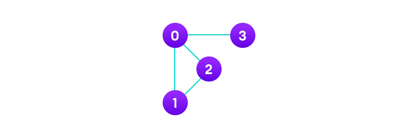
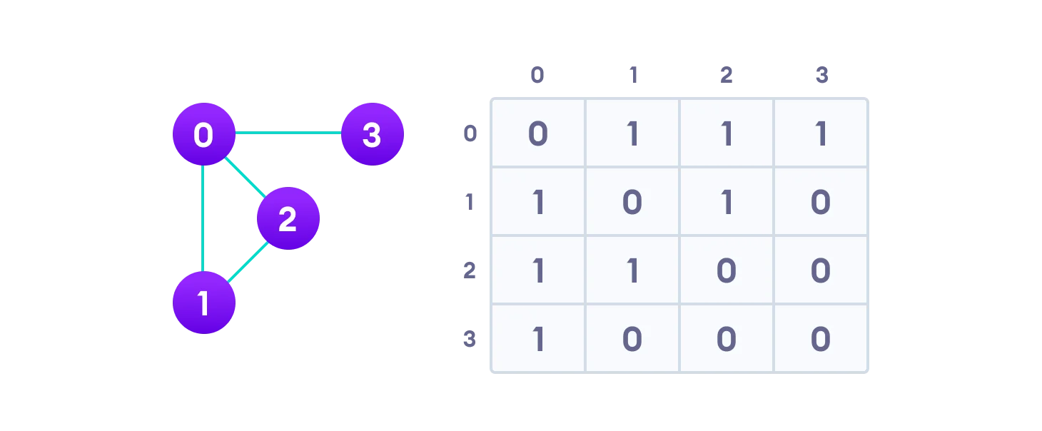
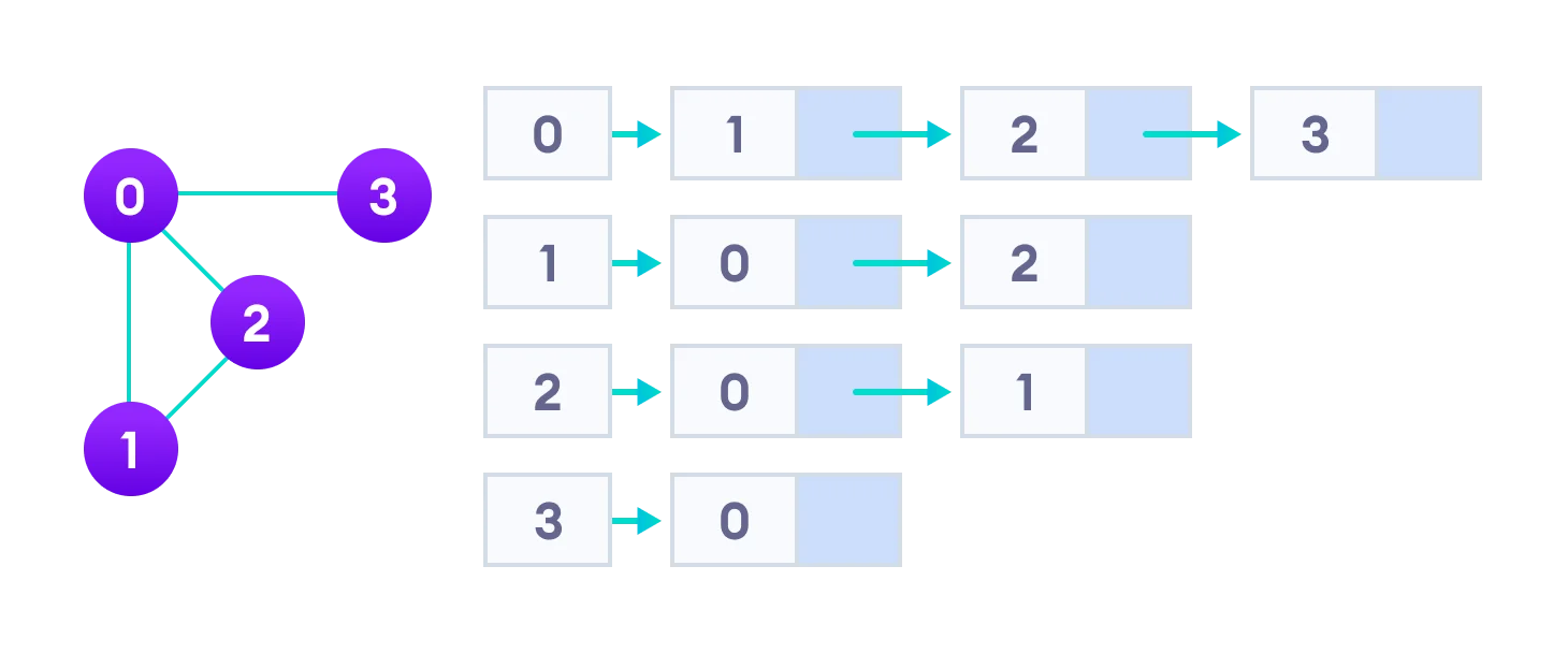
 In the graph:

 V = {0, 1, 2, 3}
 E = {(0,1), (0,2), (0,3), (1,2)}
 G = {V, E}
Graph Representation
- Adjacency Matrix: is a 2D array of V x V vertices
- Adjacency List: an array of linked lists
Types:
- Spanning Tree and Minimum Spanning Tree
The total number of spanning trees with n vertices that can be created from a complete graph is equal to n^(n-2). The edges may or may not have weights assigned to them.
A minimum spanning tree is a spanning tree in which the sum of the weight of the edges is as minimum as possible.
- Strongly Connected Components
A strongly connected component is the portion of a directed graph in which there is a path from each vertex to another vertex. It is applicable only on a directed graph.
These components can be found using Kosaraju’s Algorithm.
- Adjacency Matrix
- Adjacency List
-
Trees Data Structure
- Binary Tree
- Full Binary Tree: A full Binary tree is a special type of binary tree in which every parent node/internal node has either two or no children.
- Perfect Binary Tree: A perfect binary tree is a type of binary tree in which every internal node has exactly two child nodes and all the leaf nodes are at the same level.
- Complete Binary Tree: A complete binary tree is just like a full binary tree, but with two major differences
- Degenerate or Pathological Binary Tree: A degenerate or pathological tree is the tree having a single child either left or right.
- Skewed Binary Tree: A skewed binary tree is a pathological/degenerate tree in which the tree is either dominated by the left nodes or the right nodes.
- Balanced Binary Tree: It is a type of binary tree in which the difference between the height of the left and the right subtree for each node is either 0 or 1.
-
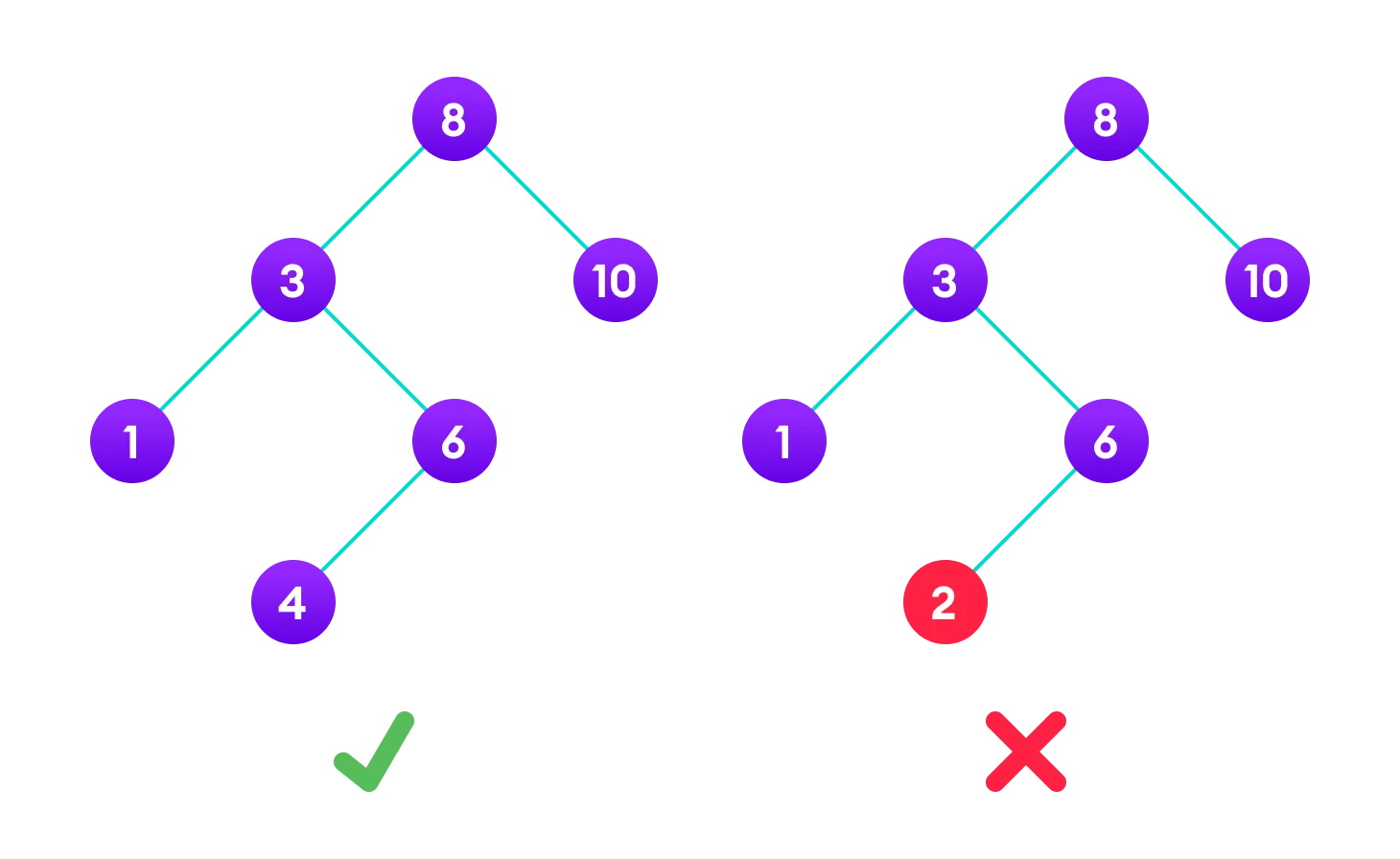
Binary Search Tree
The properties that separate a binary search tree from a regular binary tree is:
- All nodes of left subtree are less than the root node
- All nodes of right subtree are more than the root node
- Both subtrees of each node are also BSTs i.e. they have the above two properties
In the graph below, The binary tree on the right isn’t a binary search tree because the right subtree of the node “3” contains a value smaller than it.
-
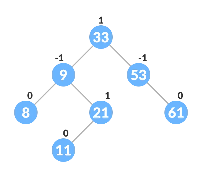
AVL Tree
AVL tree is a self-balancing binary search tree in which each node maintains extra information called a balance factor whose value is either -1, 0 or +1.
Balance Factor = (Height of Left Subtree - Height of Right Subtree) or (Height of Right Subtree - Height of Left Subtree)
AVL tree got its name after its inventor Georgy Adelson-Velsky and Landis.
An example of a balanced avl tree is
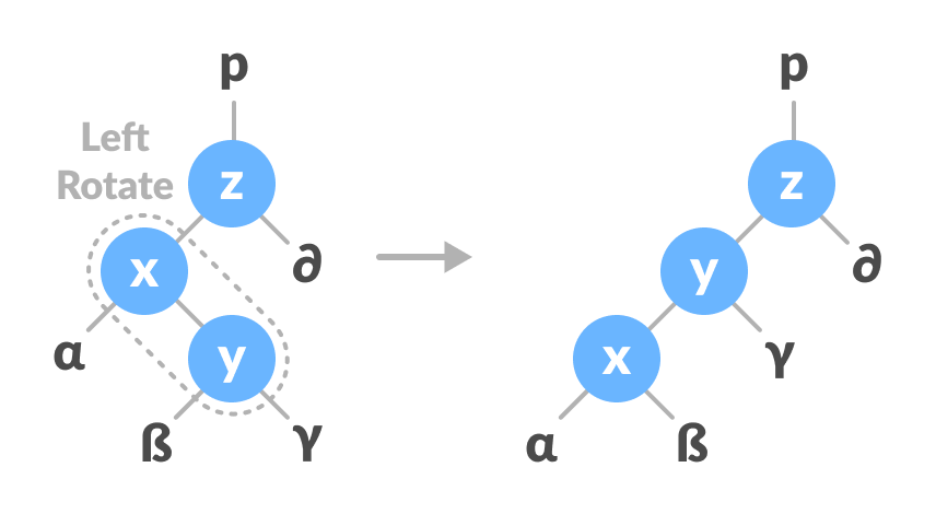
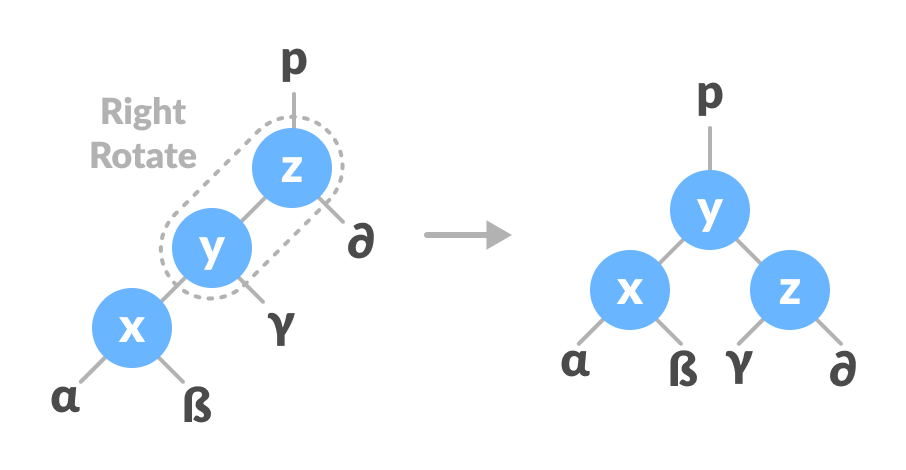
Left-Right and Right-Left Rotate:
-
B-Tree
B-tree is a special type of self-balancing search tree in which each node can contain more than one key and can have more than two children. It is also known as a height-balanced m-way tree.
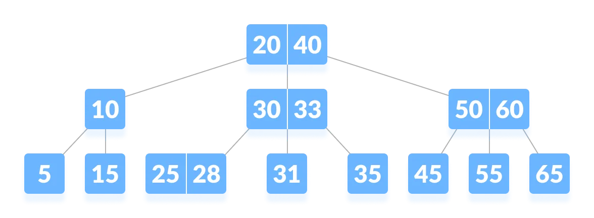
The order of the tree represents the maximum number of children a tree’s node could have. So when we say we have a B-Tree of order N, It means every node of that B-Tree can have a maximum of N children. For example, _a Binary Search Tree is a tree of order 2 since each node has at most 2 children.
The degree of a tree represents the maximum degree of a node in the tree. Recall for a given node, its degree is equal to the number of its children.
Degree represents the lower bound on the number of children a node in the B Tree can have (except for the root). i.e the minimum number of children possible. Whereas the Order represents the upper bound on the number of children. ie. the maximum number possible.
B-tree of Order n Properties:
- For each node x, the keys are stored in increasing order.
- In each node, there is a boolean value x.leaf which is true if x is a leaf.
- If n is the order of the tree, each internal node can contain at most n - 1 keys along with a pointer to each child.
- Each node except root can have at most n children and at least n/2 children.
- All leaves have the same depth (i.e. height-h of the tree).
- The root has at least 2 children and contains a minimum of 1 key.
- If n ≥ 1, then for any n-key B-tree of height h and minimum degree t ≥ 2, h ≥ logt^(n+1)/2.
-
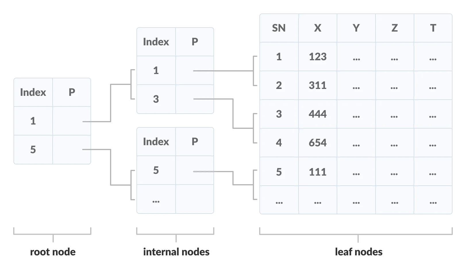
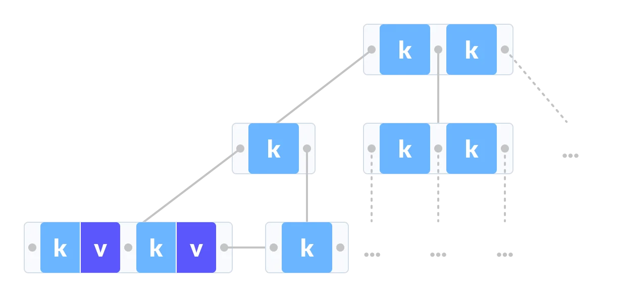
B+ Tree
An important concept to be understood before learning B+ tree is multilevel indexing. In multilevel indexing, the index of indices is created as in figure below.
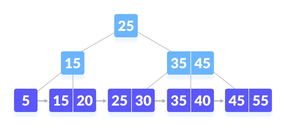
Properties of a B+ Tree of Order m:
- All leaves are at the same level.
- The root has at least 2 children.
- Each node except root can have a maximum of m children and at least m/2 children.
- Each node can contain a maximum of m - 1 keys and a minimum of ⌈m/2⌉ - 1 keys.
- Red-Black Tree
- Binary Tree
-
Linear Vs Non-linear Data Structures
| Linear Data Structures | Non Linear Data Structures |
|---|---|
| The data items are arranged in sequential order, one after the other. | The data items are arranged in non-sequential order (hierarchical manner). |
| All the items are present on the single layer. | The data items are present at different layers. |
| It can be traversed on a single run. That is, if we start from the first element, we can traverse all the elements sequentially in a single pass. | It requires multiple runs. That is, if we start from the first element it might not be possible to traverse all the elements in a single pass. |
| The memory utilization is not efficient. | Different structures utilize memory in different efficient ways depending on the need. |
| The time complexity increase with the data size. | Time complexity remains the same. |
| Example: Arrays, Stack, Queue | Example: Tree, Graph, Map |
Comparison between a B-tree and a B+ Tree
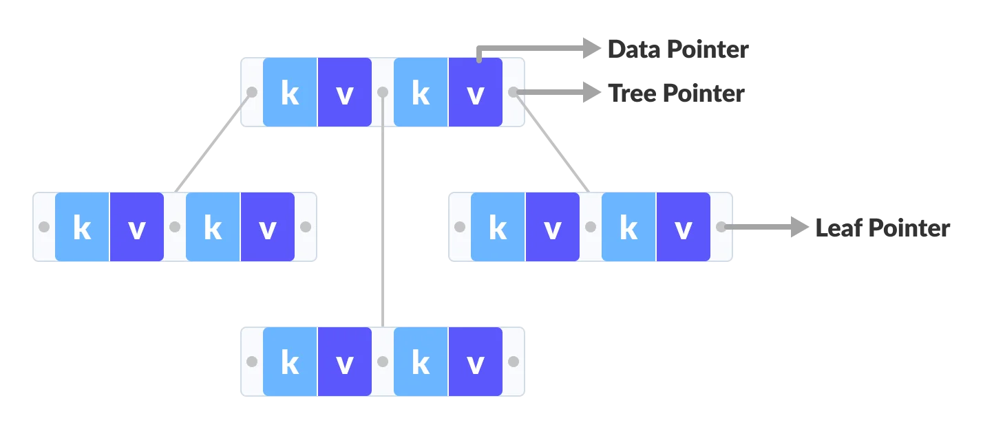
The data pointers are present only at the leaf nodes on a B+ tree whereas the data pointers are present in the internal, leaf or root nodes on a B-tree.
The leaves are not connected with each other on a B-tree whereas they are connected on a B+ tree.
Operations on a B+ tree are faster than on a B-tree.
Master Theorem
The master method is a formula for solving recurrence relations of the form:
T(n) = aT(n/b) + f(n),
where,
n = size of input
a = number of subproblems in the recursion
n/b = size of each subproblem. All subproblems are assumed to have the same size.
f(n) = cost of the work done outside the recursive call,
      which includes the cost of dividing the problem and
      cost of merging the solutions

Here, a ≥ 1 and b > 1 are constants, and f(n) is an asymptotically positive function.
Master Theorem
If a ≥ 1 and b > 1 are constants and f(n) is an asymptotically positive function, then the time complexity of a recursive relation is given by
T(n) = aT(n/b) + f(n)

where, T(n) has the following asymptotic bounds:

    1. If f(n) = O(nlogb^(a-ϵ)), then T(n) = Θ(nlogb^a).

    2. If f(n) = Θ(nlogb^a), then T(n) = Θ(nlogb^a * log n).

    3. If f(n) = Ω(nlogb^(a+ϵ)), then T(n) = Θ(f(n)).

ϵ > 0 is a constant.
Divide and Conquer Algorithm
- Divide: Divide the given problem into sub-problems using recursion.
- Conquer: Solve the smaller sub-problems recursively. If the subproblem is small enough, then solve it directly.
- Combine: Combine the solutions of the sub-problems that are part of the recursive process to solve the actual problem.
Applications:
- Binary Search
- Merge Sort
- Quick Sort
- Strassen’s Matrix multiplication
- Karatsuba Algorithm
Advantages:
- The complexity for the multiplication of two matrices using the naive method is O(n3), whereas using the divide and conquer approach (i.e. Strassen’s matrix multiplication) is O(n^2.8074). This approach also simplifies other problems, such as the Tower of Hanoi.
- This approach is suitable for multiprocessing systems.
- It makes efficient use of memory caches.
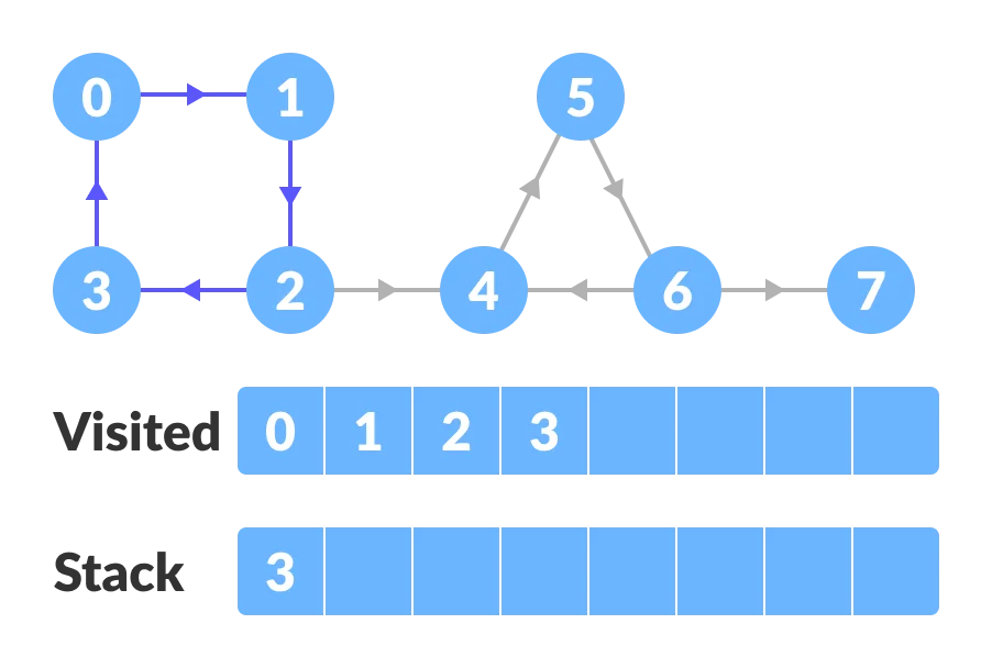
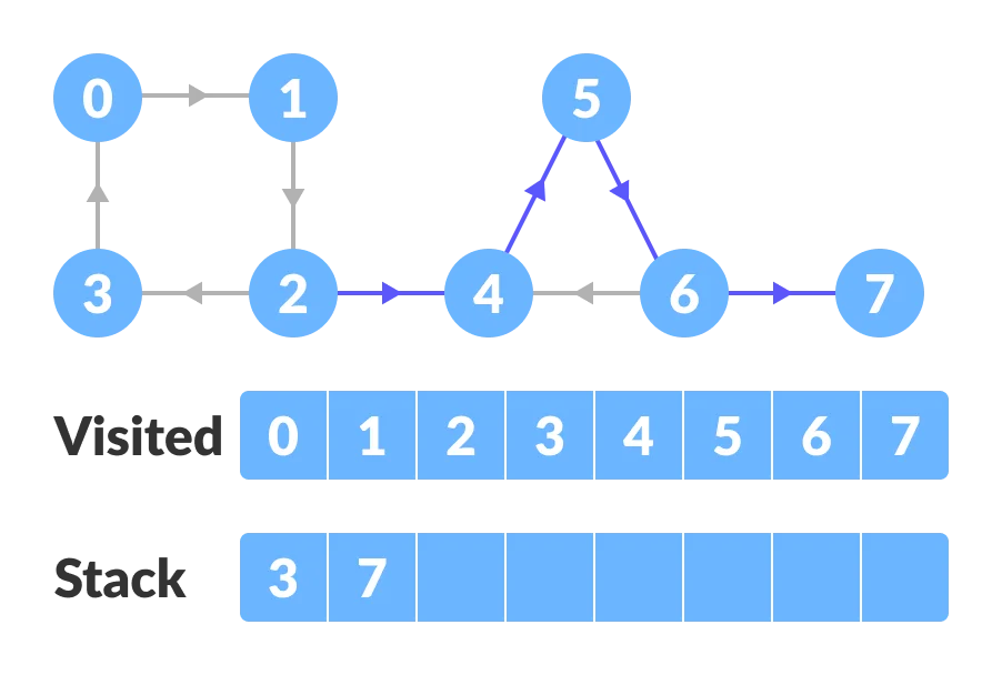
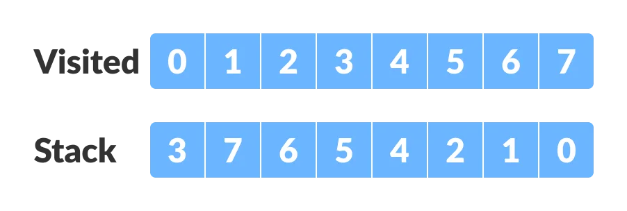
Depth First Search (DFS) Algorithm
Depth first Search or Depth first traversal is a recursive algorithm for searching all the vertices of a graph or tree data structure.
The purpose of the algorithm is to mark each vertex as visited while avoiding cycles.
The DFS algorithm works as follows:
- Start by putting any one of the graph’s vertices on top of a stack.
- Take the top item of the stack and add it to the visited list.
- Create a list of that vertex’s adjacent nodes. Add the ones which aren’t in the visited list to the top of the stack.
- Keep repeating steps 2 and 3 until the stack is empty.
Let’s see how the Depth First Search algorithm works with an example.
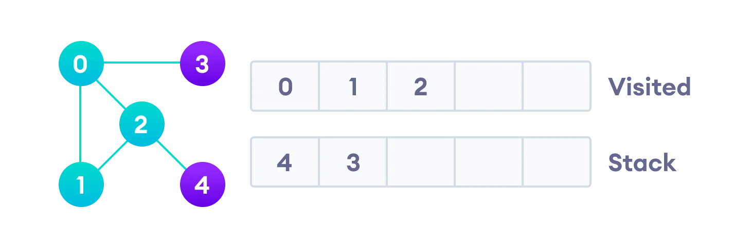
We use an undirected graph with 5 vertices.
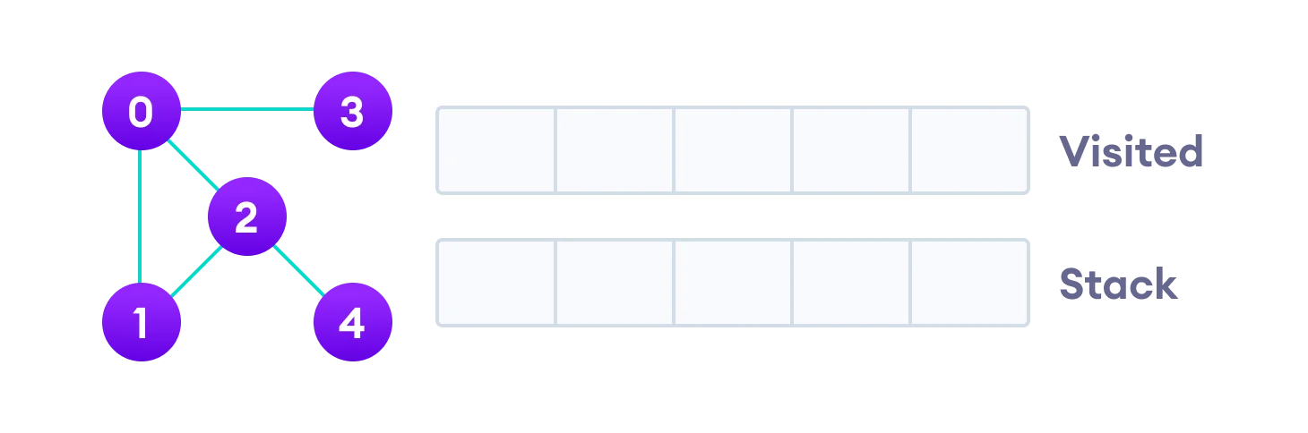
We start from vertex 0, the DFS algorithm starts by putting it in the Visited list and putting all its adjacent vertices in the stack (Last In First Out).
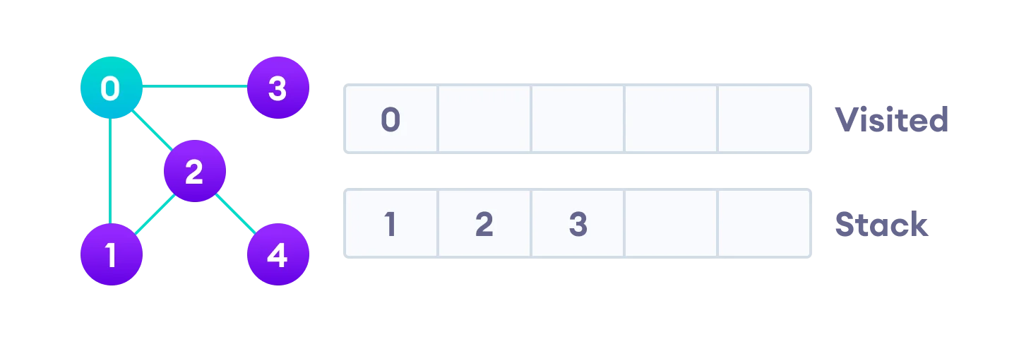
Next, we visit the element at the top of stack i.e. 1 and go to its adjacent nodes. Since 0 has already been visited, we visit 2 instead.
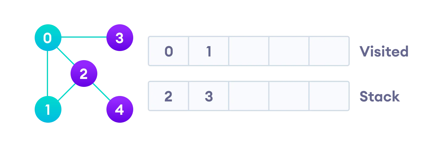
Vertex 2 has an unvisited adjacent vertex in 4, so we add that to the top of the stack and visit it.
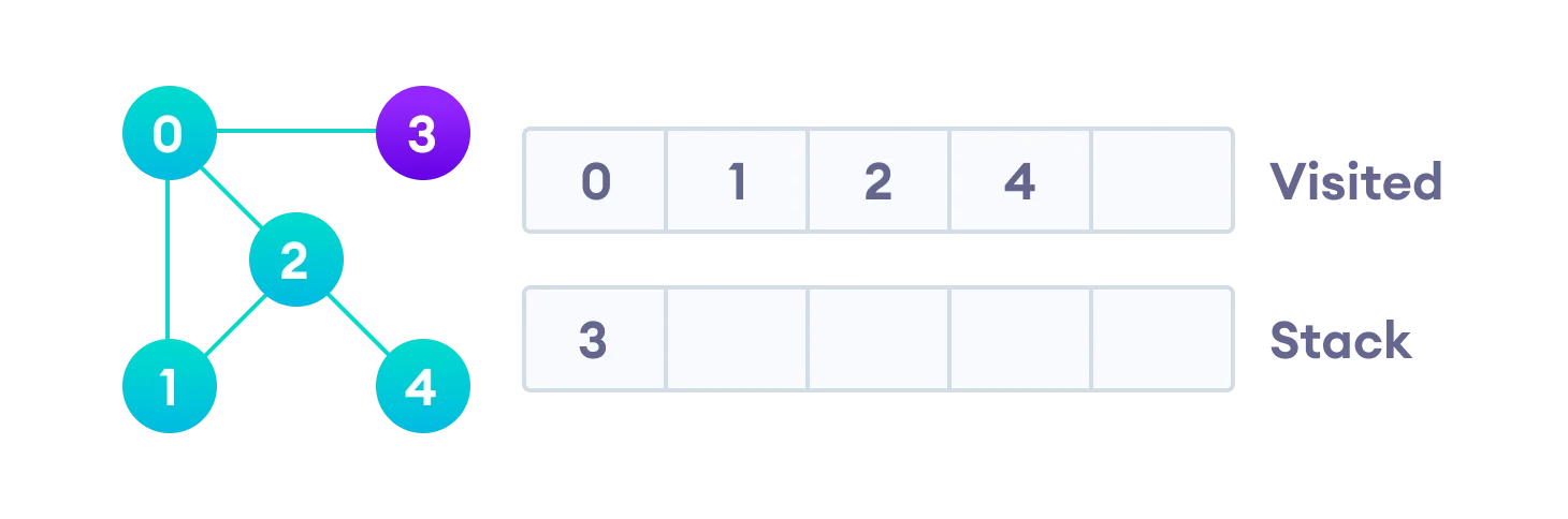
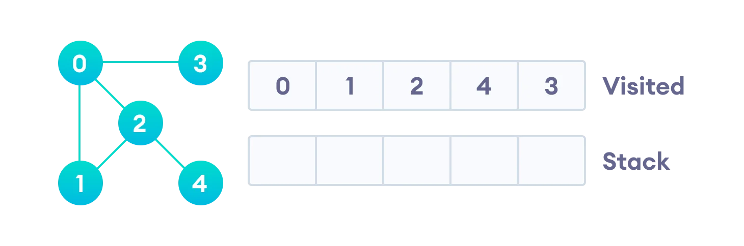
After we visit the last element 3, it doesn’t have any unvisited adjacent nodes, so we have completed the Depth First Traversal of the graph.
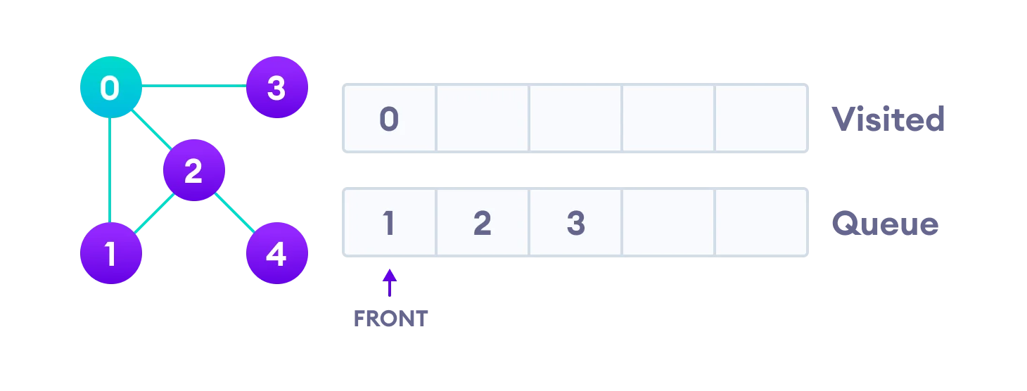
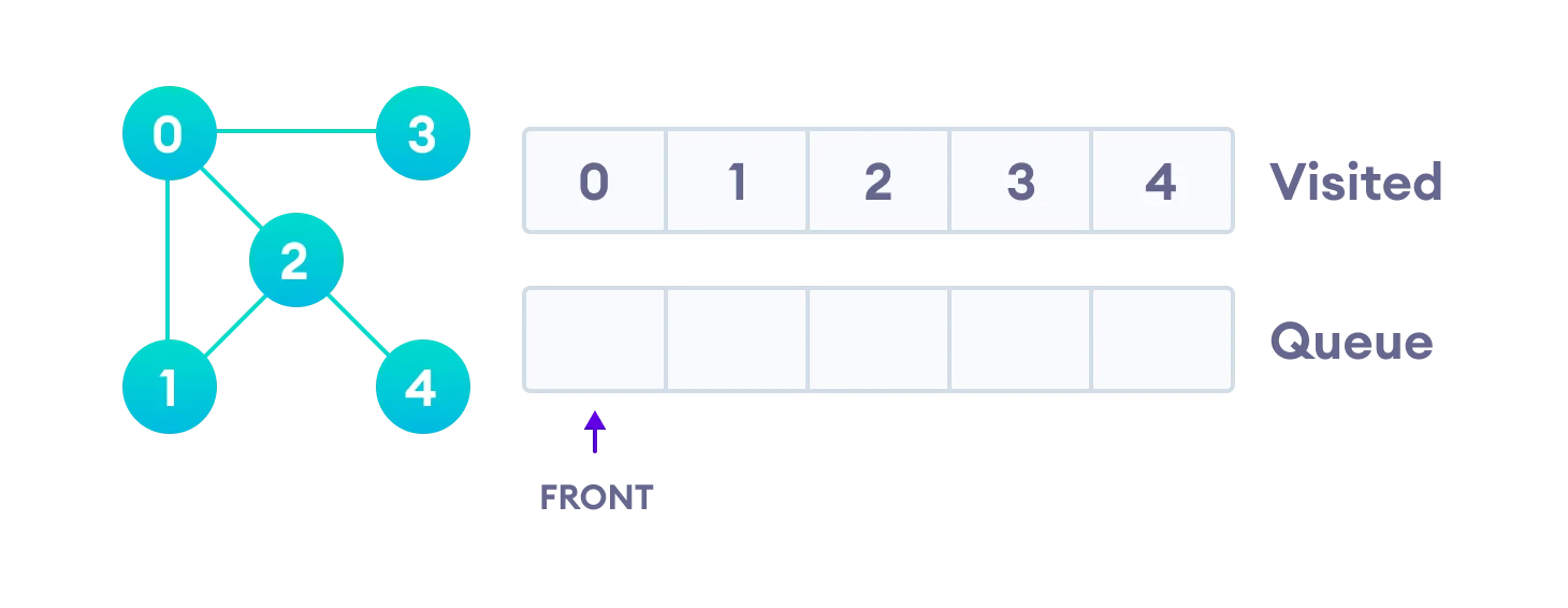
Breadth First Search (BFS) Algorithm
Breadth First Traversal or Breadth First Search is a recursive algorithm for searching all the vertices of a graph or tree data structure.
The purpose of the algorithm is to mark each vertex as visited while avoiding cycles.
The algorithm works as follows:
- Start by putting any one of the graph’s vertices at the back of a queue.
- Take the front item of the queue and add it to the visited list.
- Create a list of that vertex’s adjacent nodes. Add the ones which aren’t in the visited list to the back of the queue.
- Keep repeating steps 2 and 3 until the queue is empty.
The graph might have two different disconnected parts so to make sure that we cover every vertex, we can also run the BFS algorithm on every node. Let’s see how the Breadth First Search algorithm works with an example.
We use an undirected graph with 5 vertices.
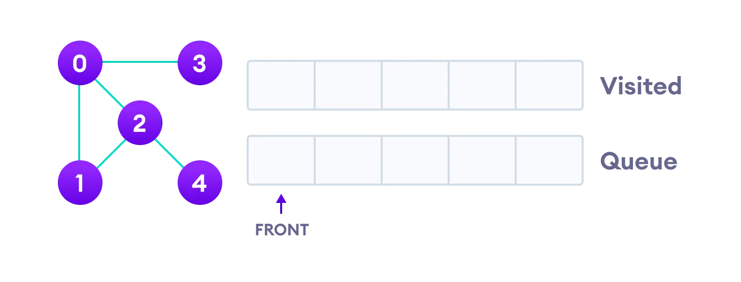
We start from vertex 0, the BFS algorithm starts by putting it in the Visited list and putting all its adjacent vertices in the queue(First In First Out).
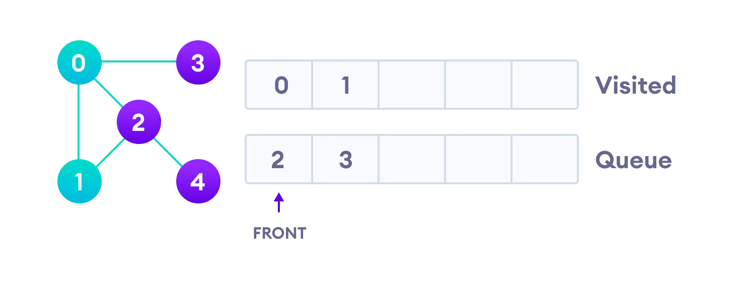
Next, we visit the element at the front of queue i.e. 1 and go to its adjacent nodes. Since 0 has already been visited, we visit 2 instead.
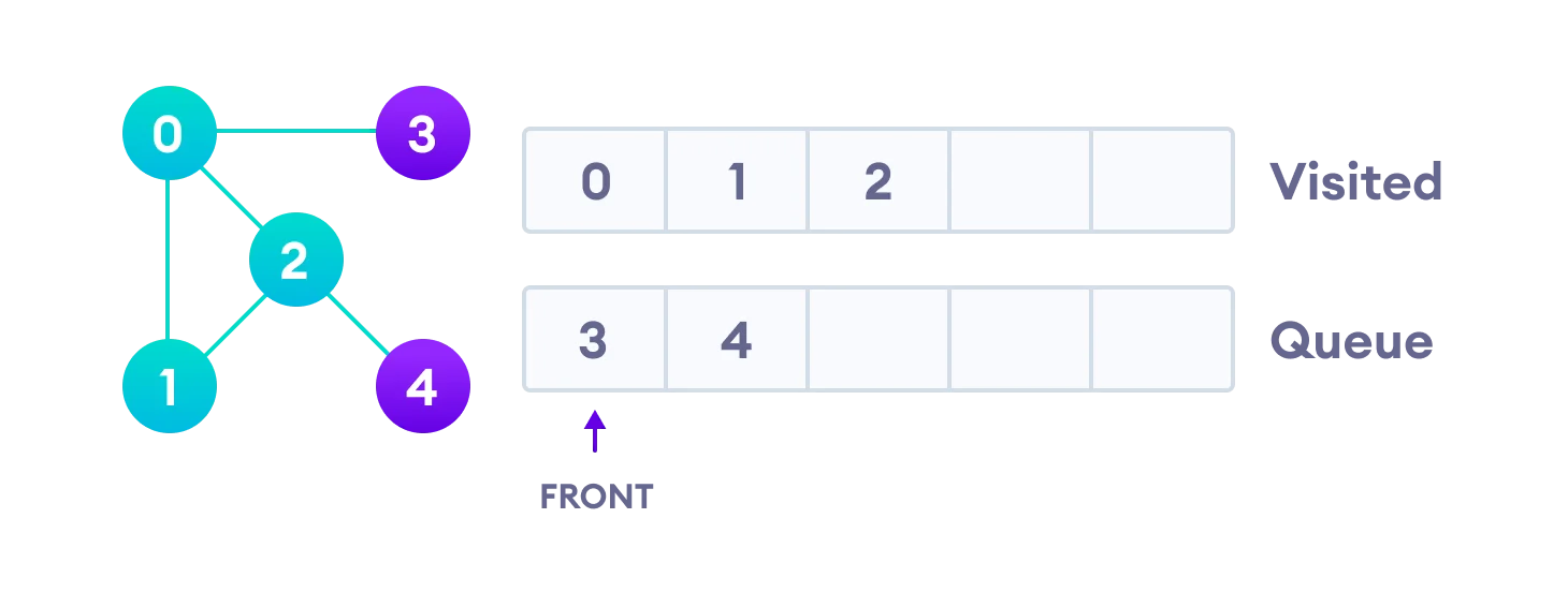
Vertex 2 has an unvisited adjacent vertex in 4, so we add that to the back of the queue and visit 3, which is at the front of the queue.
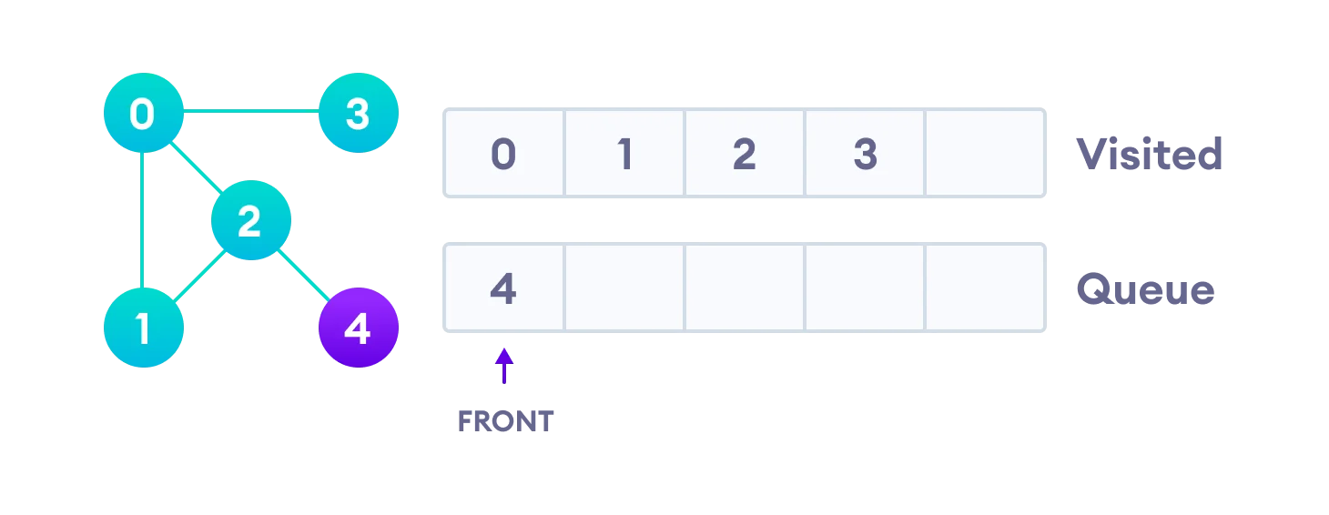
Only 4 remains in the queue since the only adjacent node of 3 i.e. 0 is already visited. We visit it.
Since the queue is empty, we have completed the Breadth First Traversal of the graph.
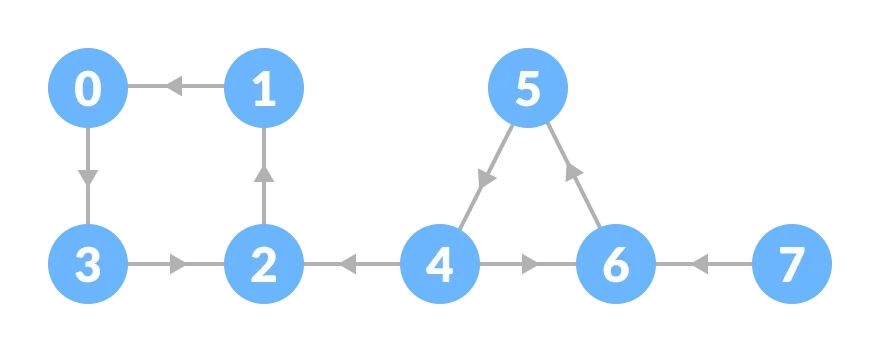
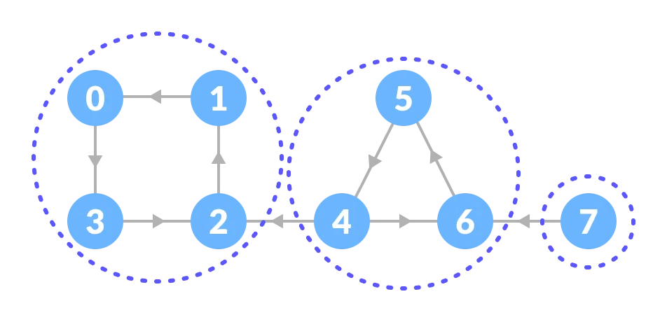
Kosaraju’s Algorithm
Kosaraju’s Algorithm is based on the depth-first search algorithm implemented twice.
Three steps are involved.
-
Perform a depth first search on the whole graph.
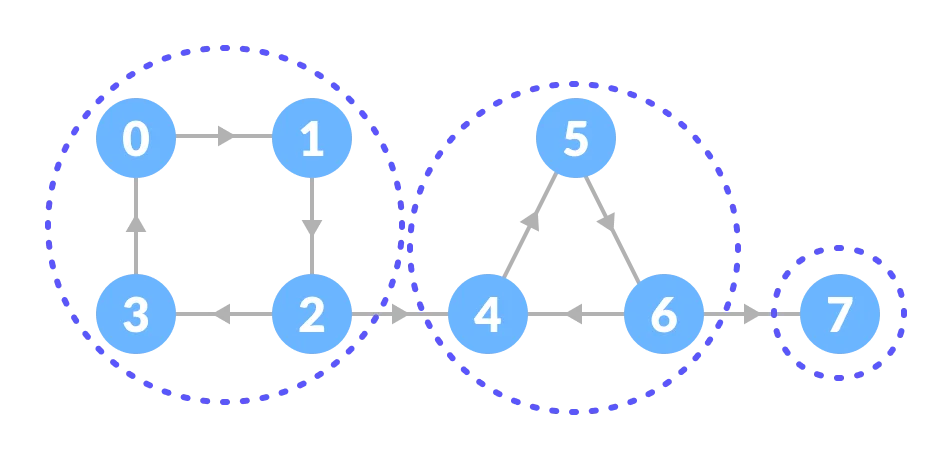
Let us start from vertex-0, visit all of its child vertices, and mark the visited vertices as done. If a vertex leads to an already visited vertex, then push this vertex to the stack.
For example: Starting from vertex-0, go to vertex-1, vertex-2, and then to vertex-3. Vertex-3 leads to already visited vertex-0, so push the source vertex (ie. vertex-3) into the stack.
Go to the previous vertex (vertex-2) and visit its child vertices i.e. vertex-4, vertex-5, vertex-6 and vertex-7 sequentially. Since there is nowhere to go from vertex-7, push it into the stack.
Go to the previous vertex (vertex-6) and visit its child vertices. But, all of its child vertices are visited, so push it into the stack.

Similarly, a final stack is created.
-
Reverse the original graph.
-
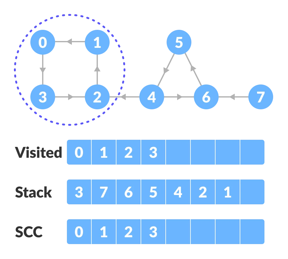
Perform depth-first search on the reversed graph.
Start from the top vertex of the stack. Traverse through all of its child vertices. Once the already visited vertex is reached, one strongly connected component is formed.
For example: Pop vertex-0 from the stack. Starting from vertex-0, traverse through its child vertices (vertex-0, vertex-1, vertex-2, vertex-3 in sequence) and mark them as visited. The child of vertex-3 is already visited, so these visited vertices form one strongly connected component (SCC).
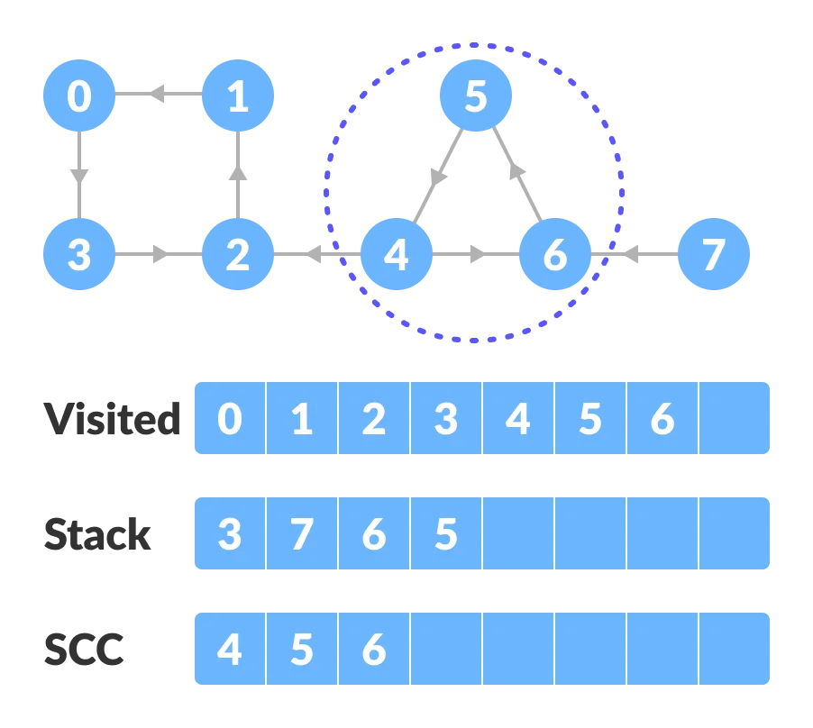
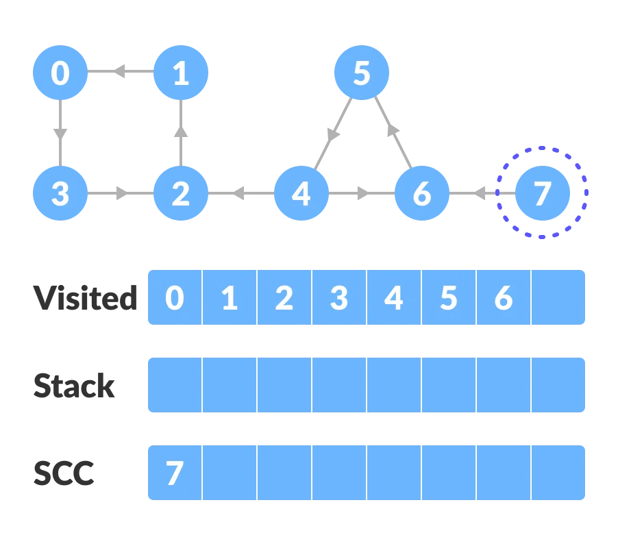
Go to the stack and pop the top vertex if already visited. Otherwise, choose the top vertex from the stack and traverse through its child vertices as presented above.
-
Thus, the strongly connected components are:
Breadth-First Search vs Depth First Search
| No. | Parameters | BFS | DFS |
|---|---|---|---|
| 1. | Stands for | BFS stands for Breadth First Search. | DFS stands for Depth First Search. |
| 2. | Data Structure | BFS(Breadth First Search) uses Queue data structure for finding the shortest path. | DFS(Depth First Search) uses Stack data structure. |
| 3. | Definition | BFS is a traversal approach in which we first walk through all nodes on the same level before moving on to the next level. | DFS is also a traversal approach in which the traverse begins at the root node and proceeds through the nodes as far as possible until we reach the node with no unvisited nearby nodes. |
| 4. | Technique | BFS can be used to find a single source shortest path in an unweighted graph because, in BFS, we reach a vertex with a minimum number of edges from a source vertex. | In DFS, we might traverse through more edges to reach a destination vertex from a source. |
| 5. | Conceptual Difference | BFS builds the tree level by level. | DFS builds the tree sub-tree by sub-tree. |
| 6. | Approach used | It works on the concept of FIFO (First In First Out). | It works on the concept of LIFO (Last In First Out). |
| 7. | Suitable for | BFS is more suitable for searching vertices closer to the given source. | DFS is more suitable when there are solutions away from source. |
| 8. | Suitability for Decision-Trees | BFS considers all neighbors first and therefore not suitable for decision-making trees used in games or puzzles. | DFS is more suitable for game or puzzle problems. We make a decision, and the then explore all paths through this decision. And if this decision leads to win situation, we stop. |
| 9. | Time Complexity | The Time complexity of BFS is O(V + E) when Adjacency List is used and O(V^2) when Adjacency Matrix is used, where V stands for vertices and E stands for edges. | The Time complexity of DFS is also O(V + E) when Adjacency List is used and O(V^2) when Adjacency Matrix is used, where V stands for vertices and E stands for edges. |
| 10. | Visiting of Siblings/ Children | Here, siblings are visited before the children. | Here, children are visited before the siblings. |
| 11. | Removal of Traversed Nodes | Nodes that are traversed several times are deleted from the queue. | The visited nodes are added to the stack and then removed when there are no more nodes to visit. |
| 12. | Backtracking | In BFS there is no concept of backtracking. | DFS algorithm is a recursive algorithm that uses the idea of backtracking |
| 13. | Applications | BFS is used in various applications such as bipartite graphs, shortest paths, etc. | DFS is used in various applications such as acyclic graphs and topological order etc. |
| 14. | Memory | BFS requires more memory. | DFS requires less memory. |
| 15. | Optimality | BFS is optimal for finding the shortest path. | DFS is not optimal for finding the shortest path. |
| 16. | Space complexity | In BFS, the space complexity is more critical as compared to time complexity. | DFS has lesser space complexity because at a time it needs to store only a single path from the root to the leaf node. |
| 17. | Speed | BFS is slow as compared to DFS. | DFS is fast as compared to BFS. |
| 18. | Tapping in loops | In BFS, there is no problem of trapping into finite loops. | In DFS, we may be trapped in infinite loops. |
| 19. | When to use? | When the target is close to the source, BFS performs better. | When the target is far from the source, DFS is preferable. |
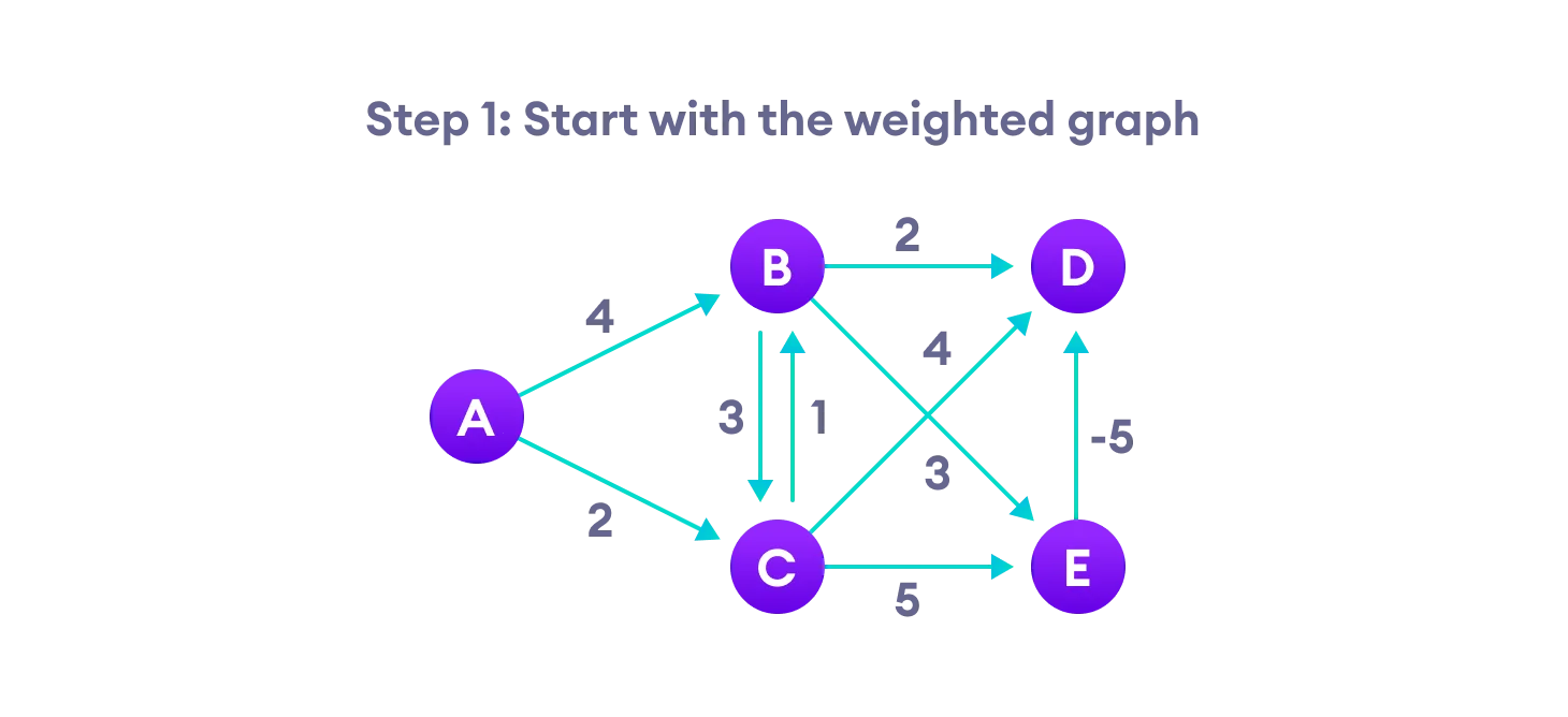
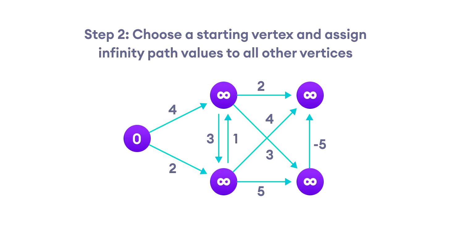
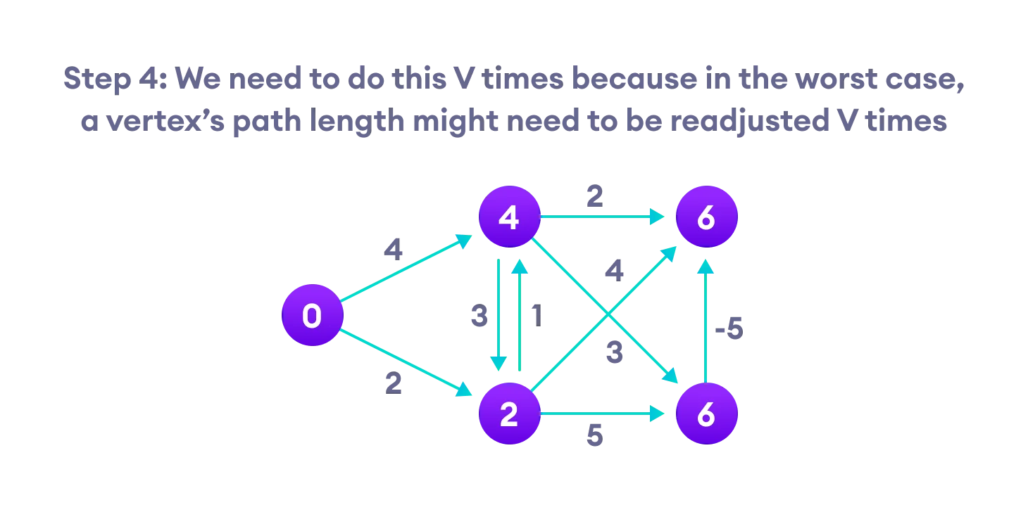
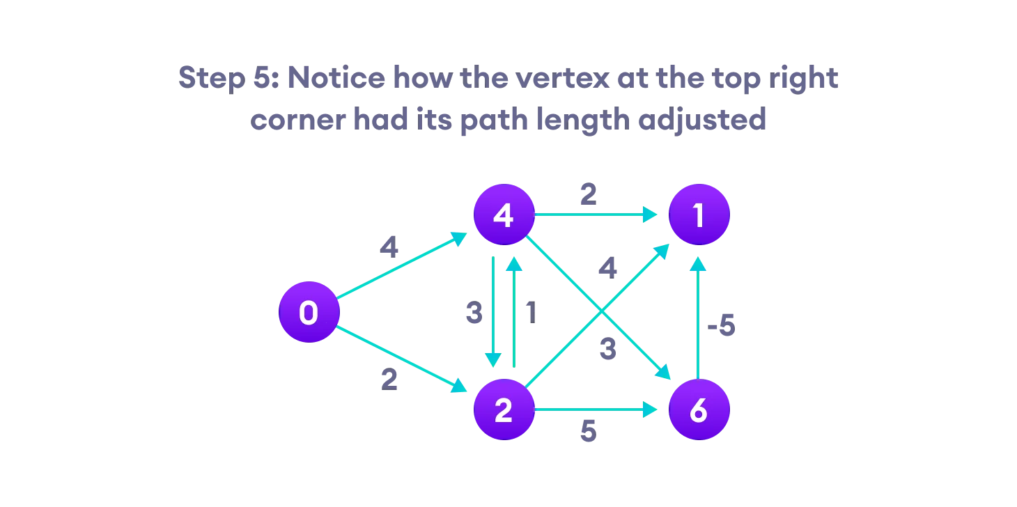
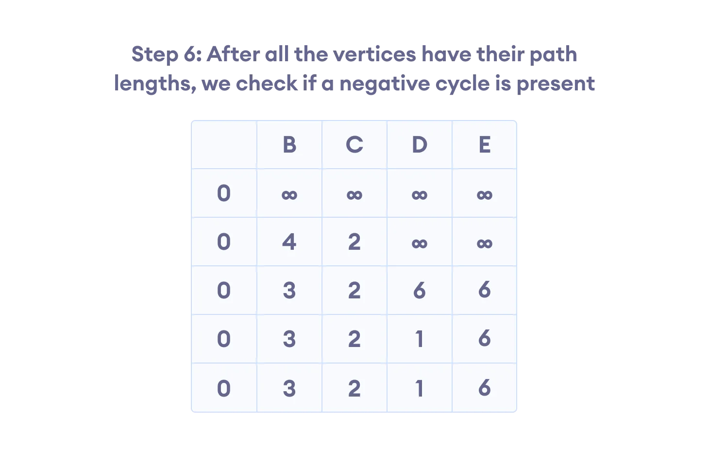
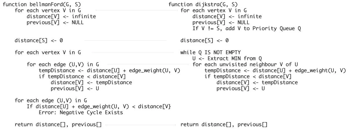
Bellman Ford’s Algorithm
Bellman Ford algorithm works by overestimating the length of the path from the starting vertex to all other vertices. Then it iteratively relaxes those estimates by finding new paths that are shorter than the previously overestimated paths.
By doing this repeatedly for all vertices, we can guarantee that the result is optimized.

Bellman Ford vs Dijkstra
Bellman Ford’s algorithm and Dijkstra’s algorithm are very similar in structure. While Dijkstra looks only to the immediate neighbors of a vertex, Bellman goes through each edge in every iteration.
Sorting and Searching Algorithms
-
Bubble Sort
Bubble sort is a sorting algorithm that compares two adjacent elements and swaps them until they are in the intended order.
- Time Complexity: Best Case = Ω(N), Worst Case = O(N^2), Average Case = Θ(N^2)
- Space Complexity: Worst Case = O(1)
-
Selection Sort
Selection sort is a sorting algorithm that selects the smallest element from an unsorted list in each iteration and places that element at the beginning of the unsorted list.
# Selection sort in Python def selectionSort(array, size): for step in range(size): min_idx = step for i in range(step + 1, size): # to sort in descending order, change > to < in this line # select the minimum element in each loop if array[i] < array[min_idx]: min_idx = i # put min at the correct position (array[step], array[min_idx]) = (array[min_idx], array[step]) data = [-2, 45, 0, 11, -9] size = len(data) selectionSort(data, size) print('Sorted Array in Ascending Order:') print(data)- Time Complexity: Best Case = Ω(N^2), Worst Case = O(N^2), Average Case = Θ(N^2)
- Space Complexity: Worst Case = O(1)
-
Insertion Sort
Insertion sort is a sorting algorithm that places an unsorted element at its suitable place in each iteration.
# Insertion sort in Python def insertionSort(array): for step in range(1, len(array)): key = array[step] j = step - 1 # Compare key with each element on the left of it until an element smaller than it is found # For descending order, change key<array[j] to key>array[j]. while j >= 0 and key < array[j]: array[j + 1] = array[j] j = j - 1 # Place key at after the element just smaller than it. array[j + 1] = key data = [9, 5, 1, 4, 3] insertionSort(data) print('Sorted Array in Ascending Order:') print(data)- Time Complexity: Best Case = Ω(N), Worst Case = O(N^2), Average Case = Θ(N^2)
- Space Complexity: Worst Case = O(1)
-
Merge Sort
Merge Sort is one of the most popular sorting algorithms that is based on the principle of Divide and Conquer Algorithm.
Here, a problem is divided into multiple sub-problems. Each sub-problem is solved individually. Finally, sub-problems are combined to form the final solution.
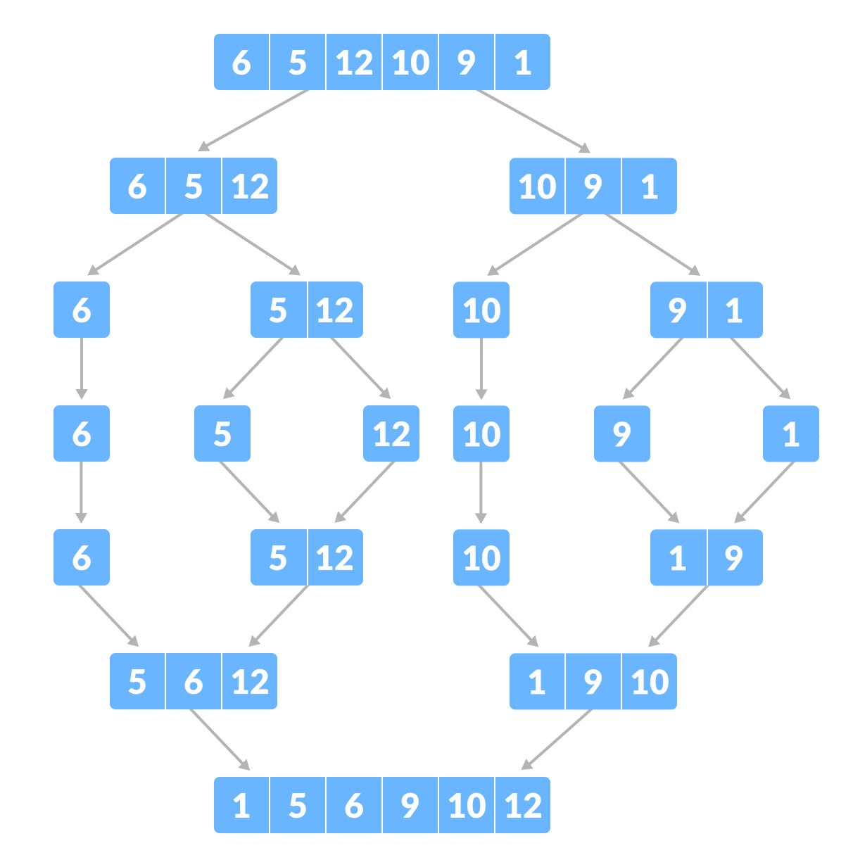
# MergeSort in Python def mergeSort(array): if len(array) > 1: # r is the point where the array is divided into two subarrays r = len(array)//2 L = array[:r] M = array[r:] # Sort the two halves mergeSort(L) mergeSort(M) i = j = k = 0 # Until we reach either end of either L or M, pick larger among # elements L and M and place them in the correct position at A[p..r] while i < len(L) and j < len(M): if L[i] < M[j]: array[k] = L[i] i += 1 else: array[k] = M[j] j += 1 k += 1 # When we run out of elements in either L or M, # pick up the remaining elements and put in A[p..r] while i < len(L): array[k] = L[i] i += 1 k += 1 while j < len(M): array[k] = M[j] j += 1 k += 1 # Print the array def printList(array): for i in range(len(array)): print(array[i], end=" ") print() # Driver program if __name__ == '__main__': array = [6, 5, 12, 10, 9, 1] mergeSort(array) print("Sorted array is: ") printList(array)- Time Complexity: Best Case = Ω(n log(n)), Worst Case = O(n log(n)), Average Case = Θ(n log(n))
- Space Complexity: Worst Case = O(n)
-
Quicksort
Quicksort is a sorting algorithm based on the divide and conquer approach where
- An array is divided into subarrays by selecting a pivot element (element selected from the array). While dividing the array, the pivot element should be positioned in such a way that elements less than pivot are kept on the left side and elements greater than pivot are on the right side of the pivot.
- The left and right subarrays are also divided using the same approach. This process continues until each subarray contains a single element.
- At this point, elements are already sorted. Finally, elements are combined to form a sorted array.
- Time Complexity: Best Case = Ω(n log(n)), Worst Case = O(n^2), Average Case = Θ(n log(n))
- Space Complexity: Worst Case = O(n)
-
Counting Sort
Counting sort is a sorting algorithm that sorts the elements of an array by counting the number of occurrences of each unique element in the array. The count is stored in an auxiliary array and the sorting is done by mapping the count as an index of the auxiliary array.
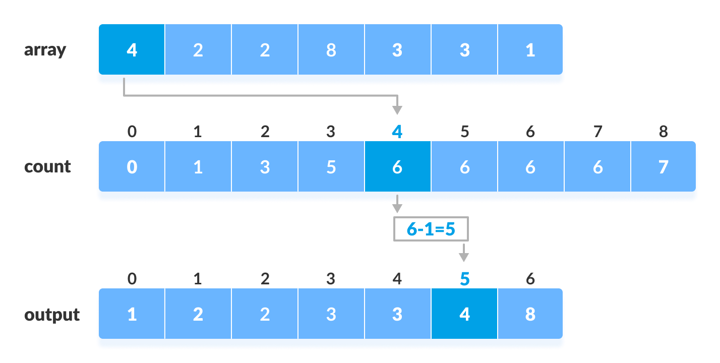
def counting_sort(array): """ Counting sort is a sorting algorithm that sorts the elements of an array by counting the number of occurrences of each element. Args: array: The array to be sorted. Returns: A sorted array. """ # Find the maximum element in the array. max_element = max(array) size = len(array) # Create a count array to store the number of occurrences of each element. count_array = [0] * (max_element + 1) # Increment the count of each element in the count array. for element in array: count_array[element] += 1 # For each element in the countArray, sum up its value with the value of the previous # element, and then store that value as the value of the current element for i in range(1, max_element + 1): count_array[i] += count_array[i - 1] # Create a sorted array by adding the elements from the count array. sorted_array = [0] * size i = size - 1 while i >= 0: sorted_array[count_array[current_element] - 1] = array[i] count_array[array[i]] -= 1 i -= 1 return sorted_array- Time Complexity: Best Case = Ω(n + k), Worst Case = O(n + k), Average Case = Θ(n + k)
- Space Complexity: Worst Case = O(k)
-
Radix Sort+
Radix sort is a sorting algorithm that sorts the elements by first grouping the individual digits of the same place value. Then, sort the elements according to their increasing/decreasing order.
- Time Complexity: Best Case = Ω(nk), Worst Case = O(nk), Average Case = Θ(nk)
- Space Complexity: Worst Case = O(n + k)
- Bucket Sort
- Heap Sort
- Shell Sort
- Linear Search
- Binary Search
Time Complexities of all Sorting Algorithms
| Algorithm | Time Complexity | Space Complexity | ||
|---|---|---|---|---|
| – | Best | Average | Worst | Worst |
| Selection Sort | Ω(n^2) | θ(n^2) | O(n^2) | O(1) |
| Bubble Sort | Ω(n) | θ(n^2) | O(n^2) | O(1) |
| Insertion Sort | Ω(n) | θ(n^2) | O(n^2) | O(1) |
| Heap Sort | Ω(n log(n)) | θ(n log(n)) | O(n log(n)) | O(1) |
| Quick Sort | Ω(n log(n)) | θ(n log(n)) | O(n^2) | O(n) |
| Merge Sort | Ω(n log(n)) | θ(n log(n)) | O(n log(n)) | O(n) |
| Bucket Sort | Ω(n + k) | θ(n + k) | O(n^2) | O(n) |
| Radix Sort | Ω(nk) | θ(nk) | O(nk) | O(n + k) |
| Count Sort | Ω(n + k) | θ(n + k) | O(n + k) | O(k) |
| Shell Sort | Ω(n log(n)) | θ(n log(n)) | O(n^2) | O(1) |
| Tim Sort | Ω(n) | θ(n log(n)) | O(n log (n)) | O(n) |
| Tree Sort | Ω(n log(n)) | θ(n log(n)) | O(n^2) | O(n) |
| Cube Sort | Ω(n) | θ(n log(n)) | O(n log(n)) | O(n) |
Greedy Algorithm
A greedy algorithm is an approach for solving a problem by selecting the best option available at the moment. It doesn’t worry whether the current best result will bring the overall optimal result.
The algorithm never reverses the earlier decision even if the choice is wrong. It works in a top-down approach.
- To begin with, the solution set (containing answers) is empty.
- At each step, an item is added to the solution set until a solution is reached.
- If the solution set is feasible, the current item is kept.
- Else, the item is rejected and never considered again.
Ford-Fulkerson Algorithm
Ford-Fulkerson algorithm is a greedy approach for calculating the maximum possible flow in a network or a graph.
A term, flow network, is used to describe a network of vertices and edges with a source (S) and a sink (T). Each vertex, except S and T, can receive and send an equal amount of stuff through it. S can only send and T can only receive stuff.
We can visualize the understanding of the algorithm using a flow of liquid inside a network of pipes of different capacities. Each pipe has a certain capacity of liquid it can transfer at an instance. For this algorithm, we are going to find how much liquid can be flowed from the source to the sink at an instance using the network.
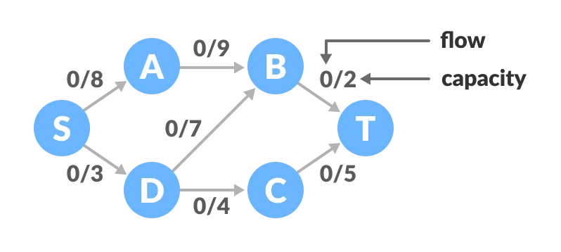
Ford-Fulkerson Algorithm for Maximum Flow Problem
Augmenting Path: It is the path available in a flow network.
Residual Graph: It represents the flow network that has additional possible flow.
Residual Capacity: It is the capacity of the edge after subtracting the flow from the maximum capacity.
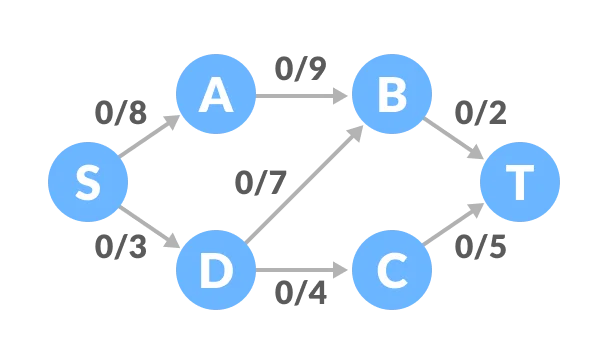
- Initialize the flow in all the edges to 0.
- While there is an augmenting path between the source and the sink, add this path to the flow.
- Update the residual graph.
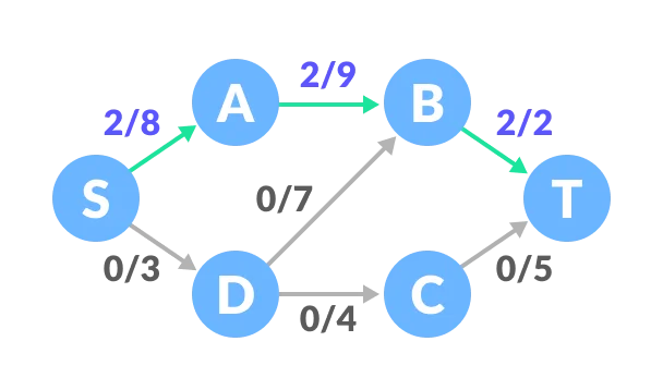
Select any arbitrary path from S to T. In this step, we have selected path S-A-B-T.
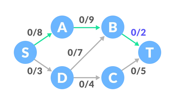
The minimum capacity among the three edges is 2 (B-T). Based on this, update the flow/capacity for each path.
Select another path S-D-C-T. The minimum capacity among these edges is 3 (S-D).
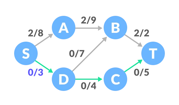
Update the capacities according to this.
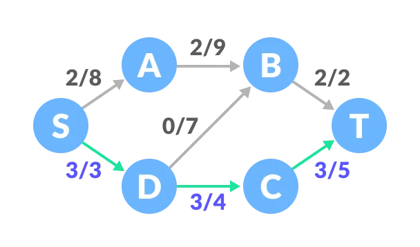
Now, let us consider the reverse-path B-D as well. Selecting path S-A-B-D-C-T. The minimum residual capacity among the edges is 1 (D-C).
Updating the capacities.
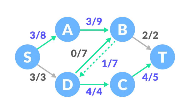
The capacity for forward and reverse paths are considered separately.
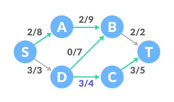
Adding all the flows = 2 + 3 + 1 = 6, which is the maximum possible flow on the flow network.
Note that if the capacity for any edge is full, then that path cannot be used.
Dijkstra’s Algorithm
Dijkstra’s algorithm is a popular search algorithm used to determine the shortest path between two nodes in a graph. Recall that Dijkstra’s algorithm operates on graphs, meaning that it can address a problem only if it can be represented in a graph-like structure.
There are several paths from Reykjavik to Belgrade that go through other cities:
- Reykjavik –> Oslo –> Berlin –> Belgrade
- Reykjavik –> London –> Berlin –> Rome –> Athens –> Belgrade
- Reykjavik –> London –> Berlin –> Rome –> Athens –> Moscow –> Belgrade
Each of these paths end in Belgrade, but they all have different values.
Before diving into the code, let’s start with a high-level illustration of Dijkstra’s algorithm.
First, we initialize the algorithm as follows:
- We set Reykjavik as the starting node.
- We set the distances between Reykjavik and all other cities to infinity, except for the distance between Reykjavik and itself, which we set to 0.
After that, we iteratively execute the following steps:
- We choose the node with the smallest value as the “current node” and visit all of its neighboring nodes. As we visit each neighbor, we update their tentative distance from the starting node.
- Once we visit all of the current node’s neighbors and update their distances, we mark the current node as “visited.” Marking a node as “visited” means that we’ve arrived at its final cost.
- We go back to step one. The algorithm loops until it visits all the nodes in the graph.
In our example, we start by marking Reykjavik as the “current node” since its value is 0. We proceed by visiting Reykjavik’s two neighboring nodes: London and Oslo. At the beginning of the algorithm, their values are set to infinity, but as we visit the nodes, we update the value for London to 4, and Oslo to 5.
We then mark Reykjavik as “visited.” We know that its final cost is zero, and we don’t need to visit it again. We continue with the next node with the lowest value, which is London.
We visit all of London’s neighboring nodes which we haven’t marked as “visited.” London’s neighbors are Reykjavik and Berlin, but we ignore Reykjavik because we’ve already visited it. Instead, we update Berlin’s value by adding the value of the edge connecting London and Berlin (3) to the value of London (4), which gives us a value of 7.
We mark London as visited and choose the next node: Oslo. We visit Oslo’s neighbors and update their values. It turns out that we can better reach Berlin through Oslo (with a value of 6) than through London, so we update its value accordingly. We also update the current value of Moscow from infinity to 8.
We mark Oslo as “visited” and update its final value to 5. Between Berlin and Moscow, we choose Berlin as the next node because its value (6) is lower than Moscow’s (8). We proceed as before: We visit Rome and Belgrade and update their tentative values, before marking Berlin as “visited” and moving on to the next city.
Note that we’ve already found a path from Reykjavik to Belgrade with a value of 15! But is it the best one?
Ultimately, it’s not. We’ll skip the rest of the steps, but you get the drill. The best path turns out to be:
- Reykjavik –> Oslo –> Berlin –> Rome –> Athens –> Belgrade, with a value of 11.